It was reported last week that a Republican working group is considering a proposal to link spending caps to the growth of actual or potential GDP. This is encouraging, and much more economically sensible than rigid balanced budget legislation.
I’ll write about other countries’ experiences with backward-looking rules in the future. But one country which uses forward-looking estimates of potential GDP to determine overall government spending is Chile. Indeed, economists such as Jeffrey Frankel have previously written glowingly about Chile’s fiscal rule, which Frankel concluded had constrained government debt whilst being flexible enough to allow automatic stabilizers to operate.
First, some background: in 2000 the Chilean government voluntarily adopted a structural budget surplus rule of one percent of GDP each year. This was lowered to half a percent of GDP in 2007, and then to a simple balanced structural budget rule in 2009 once government debt had essentially been paid off.
What does this mean in practice? A committee of independent experts meets once a year to provide the government with estimates of potential GDP. A separate committee assesses whether copper prices (a key driver of revenues) are higher or lower than trend. These two opinions are put together to determine an estimate of government revenues for the year if the economy was operating at its potential with copper prices at their long-term level. This determines the total maximum spending level allowed in the budget plan for the year. In other words, spending is capped based upon an estimate of tax revenues if the economy was at potential.
Unlike strict balanced budget proposals, the Chilean rule allows automatic stabilizers to operate, and the overall budget balance to fluctuate with the state of the economy. The government runs a deficit if output and revenues are below potential, and run a surplus if output and revenues rise above potential. Debt therefore acts a shock absorber for unforeseen deviations in economic activity. Provided the potential of the economy is estimated accurately, this means a balanced budget over the economic cycle. With economic growth then, such a rule theoretically means the debt-to-GDP ratio should gradually fall.
Crucial to the rule’s success, then, is accurate and unbiased estimates of the economy’s potential. Chile’s independent committees are designed to mitigate against the politicization of these. It’s hoped they reduce the incentive to be overoptimistic about the economy’s potential to justify higher spending. Given this independence, under Chile’s rule there are no sanctions if within a year the structural balance requirement is breached, and no adjustment in future budgets required from worse-than-expected deficits.
How has this framework performed since implementation? Prior to the financial crisis, Chilean central government debt fell sharply as a result of running sustained structural surpluses, and Chile’s sovereign debt rating improved. In fact, even the announcement of the rule in 2000 improved Chile’s creditworthiness. Frankel shows public spending fluctuated much less than in previous decades and GDP volatility declined substantially between 2001 and 2005.
The virtues of such a rule really became apparent though just before the financial crisis. President Michele Bachelet was pressured to substantially increase government spending given sustained strong GDP growth and a high world price of copper. Yet unlike the US in the early 2000s, IMF data shows that in 2007 Chile resisted these pressures and ran an overall budget surplus of 7.9 percent of GDP, with the independent experts judging most of the strong budget performance as resulting from the economy running above its potential.
This proved prescient. By 2009, the budget had swung to a 4.2 percent deficit as the global recession hit. General government debt increased again due to this large borrowing, but Chile had been so fiscally prudent prior to the crash that even today the IMF believes general government debt is only 21.3 percent of GDP, and net debt just 1 percent of GDP.
More recently, however, some of the difficulties of the rule have been in evidence. Chile raised its corporate income tax rate from 17 to 20 percent under President Sebastian Pinera in 2011, and has since raised the rate further to 25.5 percent under President Bachelet, with the intention to provide revenues for education and social spending. But during this period of higher taxes and steep spending increases (overall spending has increased by 3.8 percentage points of GDP since 2011), annual real GDP growth has performed consistently below expectations, and copper prices have been low. The result has been unforeseen structural deficits, with gross government debt near-doubling between 2013 and 2017, and net debt drifting back into positive territory, despite a pick up in global growth.
This highlights a key challenge of linking spending to potential GDP: it can be inherently difficult to assess, particularly when major supply-side policy changes occur. Calculating “cyclically-adjusted revenues” to determine spending caps requires accurate assessment of a) the health of the economy in real time, b) the “output gap” – i.e. how far the economy is away from its potential, c) how moving to potential affects revenues. All are highly uncertain and difficult to calculate.
Despite the existence of Chile’s fiscal rule then, and previous commitments to it, slower than expected growth after the crisis saw President Sebastian Pinera downgrade its stringency – aiming to hit a target of a 1 percent of GDP structural deficit by 2014. President Bachelet, in the face of sluggish growth and structural deficits being revised upwards, then began basing fiscal targets on a trajectory for the structural deficit (which should fall by 0.25 percent of GDP per year) rather than specific levels. The IMF now believes that Chile’s slow growth reflects lower potential GDP, and that the country was running a structural deficit of 2.2 percent of GDP in 2016. S&P this year downgraded Chile’s credit rating.
Chile’s experience then clearly the strengths and weaknesses of fiscal rules based upon potential GDP. In theory, and when potential GDP is estimated accurately, a structural balance rule delivers counter-cyclical fiscal policy (the correlation between Chile’s budget surplus and real GDP growth since 2007 is 0.65, see the chart below), balances budgets over the economic cycle and leads to a gradual reduction in the debt-to-GDP ratio. Independent committees, in Chile’s case, likewise help to mitigate against politicians spending near-term budget windfalls or using them to justify more optimistic forecasts.
Chile’s Counter-Cyclical Fiscal Policy
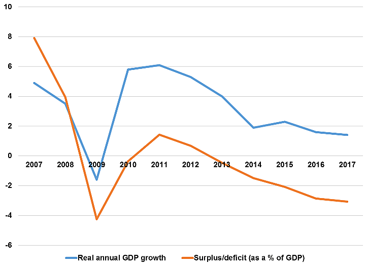
Source: International Monetary Fund Fiscal Monitor October 2017
But potential GDP is tough to measure. Under Chile’s rule, no additional constraints are placed on government spending to correct for mistakes. Ultimately, when potential GDP was revised down, and structural deficits up, successive governments chose not to adjust spending accordingly, but aimed to return to something closer to structural balance over a longer period. This highlights the limits of fiscal rules in general, and the need for political will in ensuring they are not abandoned.
The implications of letting bygones be bygones in this way and only adjusting spending decisions on a forward-looking basis might not be significant for a country starting with low levels of government debt, such as Chile. But a rule which allowed such mistakes without consequence could cause considerably more damage for a country with already high debt-to-GDP levels, such as the US.
Rules based on potential GDP are theoretically appealing and work well if estimates of potential are accurate. But that’s a big if.
