The Fiscal Impact of Immigration in the United States

This paper presents two analyses: a measure of the historical fiscal impacts of immigrants from 1994 to 2018 and the projected long‐​term fiscal impact of an additional immigrant and that immigrant’s descendants. An individual’s fiscal impact refers to the difference between the taxes that person paid and the benefits that person received over a given period. We use and compare two models for these analyses: the first follows the NAS’s methodology as closely as possible and updates the data for more recent years (hereafter referred to as the Updated Model), and the second makes several methodological changes that we believe improve the accuracy of the final results (hereafter referred to as the Cato Model). The most substantial changes made in the Cato Model include correcting for a downward bias in the estimation of immigrants’ future fiscal contributions identified by Michael Clemens in 2021, allocating the fiscal impact of U.S.-born dependents of immigrants to the second generation group, and using a predictive regression to assign future education levels to individuals who are too young to have completed their education. Other minor changes are discussed in later sections.

Immigrants have a more positive net fiscal impact than that of native‐​born Americans in most scenarios in the Updated Model and in every scenario in the Cato Model, depending on how the costs of public goods are allocated. The Cato Model finds that immigrant individuals who arrive at age 25 and who are high school dropouts have a net fiscal impact of +$216,000 in net present value terms, which does not include their descendants. Including the fiscal impact of those immigrants’ descendants reduces those immigrants’ net fiscal impact to +$57,000. By comparison, native‐​born American high school dropouts of the same age have a net fiscal impact of −$32,000 that drops to −$177,000 when their descendants are included (see Table 31). Results also differ by level of government. State and local governments often incur a less positive or even negative net fiscal impact from immigration, whereas the federal government almost always sees revenues rise above expenditures in response to immigration. With some variation and exceptions, the net fiscal impact of immigrants is more positive than it is for native‐​born Americans and positive overall for the federal and state/​local governments.

A standard complaint about immigration is that it is costly to taxpayers. Immigrants are often thought to have negative fiscal impacts, meaning they pay less in taxes than they receive in government benefits. Although the lifetime fiscal impact of an entire demographic group is difficult to measure, our results strongly imply that the opposite is true and that immigrants are a net fiscal benefit.

We used a fiscal impact model developed by the National Academy of Sciences (NAS) for its 2017 report The Economic and Fiscal Consequences of Immigration to study the fiscal impact of immigrants compared with native‐​born Americans.¹ This report explores questions such as the following: Do future immigrants arriving at a certain age and education level contribute positively or negatively to the country’s finances? Will their children pay more in taxes when they grow up than they receive in other benefits now? What is the overall impact of immigrants currently in the country compared with that of current native‐​born Americans?

The NAS fiscal impact model uses a generational accounting method to predict the fiscal impact of immigrants on the budgets of the federal and state/​local governments over a 75‐​year period. It then presents the fiscal impact in net present value (NPV) terms, discounted by 3 percent. Generational accounting measures how much each adult generation, on a per capita basis, is likely to pay in taxes net of transfer payments. NPV refers to the total lifetime fiscal impact of an individual and their potential descendants, taking into account the likelihood of survival, emigration, fertility, and other relevant factors. These methods are the best for estimating how immigrants affect government finances over their life cycles because government benefits received and taxes paid vary predictably over a person’s lifetime.² Benefits received are typically lower than taxes paid during working years and higher during childhood and old age.

The NAS model makes average fiscal projections for immigrants, depending on their age of arrival and level of education. Those projections depend on historical data and projections of future government spending levels, tax rates, economic growth, return migration, and demographics.³ We first replicated the NAS fiscal model for data from the years 1994–2013, the range for the NAS’s original research. To our knowledge, we are the first outside scholars to replicate the NAS fiscal impact model. The minor differences between our replication and the original are purely the result of revisions to the same underlying data since the publication of the NAS study in 2017, and we did not report those results for that reason. Next, we updated the NAS model to include 2014–2018 data without making changes to the NAS methodology. The results of this model, which we call the Updated Model, are similar to the original 2017 NAS study. In general, we find that the fiscal impacts of immigrants are more positive at the federal level and more negative at the state/​local level compared with native‐​born Americans. In total, we find that immigrants are more fiscally positive than native‐​born Americans.

Lastly, we constructed a model with methodological changes to the NAS model, which we call the Cato Model. We addressed a bias to immigrants’ tax receipts identified by Michael Clemens in 2021 by combining the generational accounting model with a simple economic model that accounts for the extra taxes paid by additional capital investments made in response to immigration‐​induced population growth.⁴ We also allocated the fiscal impact of U.S.-born dependents of first‐​generation immigrants to the second‐​generation group, used a predictive regression to assign future education levels to individuals who are too young to have completed their education, and made several smaller adjustments discussed in later sections. Even with those changes, the results of the Cato Model confer a similar conclusion to those produced by the Updated Model, although the NPV of the overall fiscal impact of immigrants is more positive in the Cato Model. This paper presents two analyses: a measure of the historical impacts of immigrants and the predicted long‐​term fiscal impact of an additional immigrant and that immigrant’s descendants.

We updated the NAS fiscal impact model and created a Cato Model for three reasons. The first reason was to uncover important truths about how immigrants affect government finances. The second was so the Cato Institute can become a resource for the public, policymakers, academics, members of the media, and others who want to understand how immigrants affect government finances today and in the future. Cato scholars will be able to revise the Updated Model and the Cato Model with more‐​recent data to study policy shocks and to evaluate the budgetary impact of real or proposed changes in immigration policy. The third reason was to identify how much government spending programs would have to be adjusted to improve the fiscal impact of immigration, which will be especially valuable the next time Congress considers immigration reform. Describing the fiscal impact of immigration in a format that is broadly parallel to that of the 2017 NAS report means that our text and formatting are similar to that of the 2017 NAS report. Although we endeavored to cite liberally, this paper contains half‐​sentences, sentences, or paragraphs with verbiage similar to that of the 2017 NAS report.

The fiscal impact of immigration in chapter 8 of the 2017 NAS report The Economic and Fiscal Consequences of Immigration was broken into two substantive sections. The first estimates the historical fiscal impact of immigrants from 1994 to 2013 and relies primarily on cross‐​sectional tax, income, and public expenditure data from the Annual Social and Economic Supplement (ASEC) of the Current Population Survey (CPS). The second estimates the future impact immigrants and their children will have on public finances. In addition to using CPS data, those projections use estimates of demographic changes, including education, fertility rates, life expectancies, and immigration and emigration rates. Projections of fiscal aggregates used to estimate demographic group impacts are from long‐​term budget projections produced by the Congressional Budget Office (CBO). For the historical portion of our analysis, we follow the NAS methodology, with minor alterations where better data were available. However, the CBO’s switch from 75‐​year to 30‐​year projections forced us to shorten the projected fiscal impacts by 45 years in our updated analysis, making a comparison of our findings with the 2017 study difficult, but the shorter time frame means the projections are more likely to be accurate. For context, a 75‐​year forecast of today’s budget would have been made during the Truman administration.

As in the NAS 2017 report, our immigrant and education groups are as follows: The first generation consists of foreign‐​born individuals, excluding those born abroad who gain citizenship at birth because their parents are U.S. citizens. The second generation includes U.S.-born persons with at least one foreign‐​born parent. The third‐​plus generation includes all U.S.-born persons who were born to U.S.-born parents (see Box 1). Persons with one foreign‐​born parent and one native‐​born parent are split equally between the second and third generations.⁵ The education groups are less than high school, high school graduate, some college but no college degree, college graduate, and graduate‐​level education. This educational disaggregation is necessary because fiscal impacts vary by income level, which is closely correlated with an individual’s education level.

Except in the sections involving dependents, we used individuals rather than households as the unit of measurement, which allowed us to avoid making assumptions about household composition over time and to directly measure the impact of an additional immigrant arriving in the United States. Households change through births, deaths, divorces, the departure of children, new family members arriving possibly from abroad, job losses, and other reasons. Focusing on individuals also removes the complication of multigenerational households, in which some members are immigrants and others are native born.⁶ Taxes, expenditures, and other benefits are thus assigned to the individuals who are most directly related to them. For most flows, such as personal income taxes or retirement income, this process is simple. Other flows, such as taxes jointly filed by couples or childhood education expenditures, require assumptions to allocate them to individuals. Some of those flows are allocated by program participation or by generation group. For example, federal refugee aid is split equally among all immigrants because we cannot identify refugees in the CPS. Further details on these assumptions can be found in Appendix A.

We follow the NAS 2017 construction of eight cost‐​allocation scenarios. Half the scenarios use an average‐​cost method and half a marginal‐​cost method.⁷ Theoretically, the cost to a government for providing public goods to one additional immigrant is zero. This assumption is captured under the marginal‐​cost scenarios, in which the costs of public goods—such as defense spending, subsidies, and interest payments—are assumed to be zero for individual immigrants. However, because the cost of some public goods increases with usage (i.e., congestion), the average cost method allocates these costs equally across the entire population. The scenarios are defined in Box 2.

Under Scenarios 1–4, both immigrants and native‐​born Americans pay a portion of the cost of public goods. Under Scenarios 1, 3, and 4, those public goods include defense, foreign aid, state/​local‐​level subsidies, and interest payments (both federal and state). Only natives pay those costs under Scenarios 5–8. Scenarios 2 and 6 exclude interest costs because they represent past expenditures that are not attributable to a new immigrant. Scenarios 3 and 7 reduce immigrants’ sales and consumption taxes under the assumption that immigrants send 20 percent of their income to their home countries as remittances. Scenarios 5 and 8 omit capital income taxes for immigrants who have been in the United States for less than 10 years because recent immigrants typically have lower rates of stock ownership.⁸ This paper primarily focuses on Scenarios 1 and 5 because allocating the cost of public goods affects immigrants’ fiscal impacts more than any other assumption in these scenarios.

Data for the historical fiscal cost estimates come primarily from the Current Population Survey’s Annual Social and Economic Supplement (ASEC). The CPS is a monthly household survey conducted by the Census Bureau and the Bureau of Labor Statistics that contains information on education, labor force statistics, and personal demographics. Our sample is restricted to 1994–2018 for several reasons. Before 1994, questions on birthplace, citizenship, and parental birthplace were not included in the survey. And although ASEC samples for the years 2019 and 2020 are available at the time of writing, they lack retirement income data, which are needed to estimate the fiscal impact of individuals at older ages. The household‐​level variables in the CPS are allocated among household members according to the assumptions outlined in Appendix A. Other benefits are allocated equally to individuals in a particular group, such as refugee aid to immigrants. Aggregate public expenditures are divided equally among all individuals in the sample (see Appendix A).

Some fiscal flows require alternative data sources. For public elementary and secondary school spending, we used state per‐​pupil current spending from the Census Bureau’s Annual Survey of School System Finances for the years 1994–2018.⁹ We assumed 100 percent enrollment for elementary and middle school students (ages 5–14). For high school students, we applied a half weight to those enrolled half‐​time and for elementary or junior high students (5‑to‐​14‐​year‐​olds) and assumed 100 percent enrollment. Those assumptions follow methods from the NAS 2017 report.

Because the CPS does not estimate the number of people living in institutions, we used the American Community Survey (ACS) to adjust each flow.¹⁰ This adjustment is particularly important for estimating Medicare expenditures, as a large fraction of elderly individuals live in nursing homes. We used Integrated Public Use Microdata Series ACS samples for the years 1980, 1990, and 2000–2019 and interpolated for years without a sample.¹¹ Individuals are separated into two groups depending on their immigration status. Individuals are defined as institutionalized if they live in group quarters (GQ = 3). As the ACS does not ask individuals for their parents’ birthplace, second and third‐​plus generations are not distinguishable. Institutionalized estimates were created for native‐​born Americans (second‐​plus generations). Thus, we assumed that the proportion institutionalized is the same for both second and third‐​plus generations. Population estimates are also adjusted to the Census Bureau’s reports of the annual resident population.¹²

Following the NAS 2017 approach, we adjusted each demographic group’s estimates of fiscal flows to a set of aggregate controls. Those data come from three sources: the Bureau of Economic Analysis National Income and Product Accounts, the Office of Management and Budget historical outlay tables, and health insurance data from the Centers for Medicare & Medicaid Services.¹³

For the historical analysis, we made two notable data changes from the NAS 2017 report. An important component of estimating the cost of elementary school education is English proficiency, as it is related to proportioning public school spending for English as a second language at the state and local levels. In the NAS 2017 report, schoolchildren—as surveyed by the ACS—were defined as having limited English proficiency if they were an immigrant and “did not speak English at home” or were reported to “not speak English well” or “not speak English” at all according to the definitions of the ACS’s measures of English proficiency.¹⁴ In our analysis, an immigrant schoolchild with limited English proficiency is someone who speaks English “not well” or “not at all” or “does not speak English at home” and does not speak English “well” or “very well.”¹⁵

The second change relates to the estimate of Medicare and Medicaid expenditures. Because the CPS reports Medicare and Medicaid participation but not the amount of funds received by an individual, we needed to rely on other sources. The authoritative source on national health care expenditure is the National Health Expenditure Accounts (NHEA).¹⁶ When the NAS published its 2017 report, it reported only per capita health care expenditures by age group. The NHEA now release more‐​detailed age and gender health care expenditure data. For this update, we made use of previously unavailable per‐​enrollee Medicare and Medicaid expenditures by age group and gender. Those data allowed us to more accurately allocate Medicaid funds because Medicaid is used at higher rates by young Americans. Per capita estimates are not sensitive to this distinction, as most health care is consumed by the elderly population.¹⁷

The 2017 NAS report did not include government subsidies for the purchase of health insurance on the health exchanges, also called health insurance marketplaces, as established under the Patient Protection and Affordable Care Act (ACA). The ACA health exchanges were certified and operational on January 1, 2014, so they fell outside the fiscal window of 1994–2013, as analyzed by the 2017 NAS report. CPS only began collecting data on the marketplace insurance use rates in 2019. As a result, our descriptive analysis of the net fiscal impact of immigrants and native‐​born Americans for 2014–2018 does not include that important government health care subsidy. Our back‐​of‐​the‐​envelope estimate of health insurance marketplace premium subsidies using data from the Centers for Medicare & Medicaid Services on state ACA subsidy averages and the CPS found that 3.43 percent of first‐​generation immigrants, 2.26 percent of second‐​generation immigrants, and 1.69 percent of the third‐​plus generation consumed those subsidies in 2019–2020.¹⁸ The average dollar amount for the first and second generations was $471, and the third‐​plus generation consumed $505 for the same 2019–2020 period. These calculations are too crude to include in the Updated Model or Cato Model of the current and historical net fiscal impact estimates, but they do indicate that the omission of ACA health insurance premium subsidies probably does not radically alter our results for the 2014–2018 period. However, our projections for the next 30 years include ACA subsidies because they are a component of the CBO 30‐​year fiscal outlook. Future versions of this report will include the ACA subsidies in the current and historical 2014–2018 period if and when those microdata become available.

In the estimates that follow, we explore the population and age structures of first‐​generation immigrants, the second generation, and third‐​plus generation Americans as defined previously. We then show how differences in age, education, and income affect taxes paid and benefits received. Some analysis involves allocating the costs of children and other dependents to their caregivers (see Box 3). In this case, the individual‐​level analysis does not hold, so we used a household‐​level analysis. Estimates often use single‐​year samples, whereas others use an average over three years. We chose to use single‐​year instead of three‐​year averages to smooth outliers and to keep as close as possible to the NAS 2017 methods.

The historical and current fiscal impacts of immigration on federal and state/​local government budgets do not necessarily determine the future flows, as demographic and budgetary changes will affect taxes paid and benefits received. Changes in U.S. fiscal policy, immigration policy, fertility rates, life expectancies, the age of arrival of immigrants to the United States, return emigration rates, educational attainment, and broader trends in international immigrant flows all affect the future impact that immigrants will have on U.S. government finances. We updated the NAS 2017 model that answers questions such as the following: Do future immigrants arriving at a certain age and education level contribute positively or negatively to the country’s finances? Will their children pay more in taxes when they grow up than what they receive in other benefits now? What is the impact of immigrants currently in the country compared with current native‐​born Americans?

Future estimates were made for the average person in each age, education, and immigration demographic cell. To reiterate, the education groups are less than high school, high school graduate, one to four years of college, a four‐​year college degree, and more than four years of college. For the immigration groups, we added a category for recent immigrants who arrived within the past five years. Comparing recent immigrants with all immigrants demonstrates how changes in immigrant demographics will affect fiscal flows over time. The range of the age profiles is constrained by the CPS, which has a maximum age of 80. Using fertility estimates, we also forecasted fiscal flows for the children of immigrants and native‐​born Americans. The age‐​specific fertility rates of immigrants and native‐​born Americans are calculated using the ACS’s five‐​year 2019 sample and measure the average number of births per 1,000 women of childbearing ages. We (in both the Cato Model and Updated Model) and the NAS used age‐​specific fertility rates because they are less affected by changes in the population age composition and are thus more useful for comparing subgroups over time.¹⁹

Because educational attainment has significant impacts on an individual’s tax payments and welfare receipts, we constructed a simple linear regression following the NAS method in 2017 to predict the future educational attainment of each immigrant group.²⁰ Using CPS samples, we identified a group of parents in a specific year who are at least 25 years old and thus are assumed to have completed their education and who have children aged between 10 and 16.²¹ We then identified the average education level of those children 15 years later, when they are 25 years old or older, and regressed the children’s average years of schooling on their parents’ average years of schooling. Separate regressions are done for parents born in the United States, Mexico, Central America (without Mexico), South America, Canada, Europe, Africa, East Asia, Southeast Asia, and Other Asia (Eurasia, Central Asia, and Oceania) because the impact of a parent’s education on his or her child’s education varies by region of birth.²² This process provides us with an estimate of increases in educational attainment over time, dependent on the parent’s birthplace. Additional details on this regression can be found in Appendix A.

Average tax payments and benefits for each age, education, and immigrant group are constructed using the smoothed profiles from 2016–2018 estimated in the following section. They are then extended using population projections by age and nativity from the Census Bureau’s 2017 estimates and adjusted by estimated aggregates given by the three alternative budget scenarios produced by the CBO, as defined in Box 4, until 2051.²³ Then, for each cohort—that is, ages ranging from birth to 80, the five education groups, and the three immigrant groups—the tax and benefit averages are summed and weighted by probability of survival. For immigrants, the probability of remaining in the country is also applied. For the Updated Model, we continued to use the emigration probabilities estimated by the NAS.²⁴ A discount rate of 3 percent is applied to construct final NPV flows.²⁵ The net future impact of the group for a particular age is interpreted as the discounted sum of future taxes and benefits for the group of that age in 2018 (measured in 2012 dollars), when the future projections begin.

As with the historical impact component, we constructed estimates varying the treatment of public goods. The analysis that follows includes categories that exclude all public goods; include public goods such as defense spending, subsidies, and rest‐​of‐​world payments; and include public goods covering defense spending, subsidies, rest‐​of‐​world payments, and interest payments. Congestible public goods include public administration, police, firefighting services, and incarceration costs.²⁶ Estimates excluding public goods underestimate the public benefits each demographic group receives, and estimates including public goods overestimate the public benefits each demographic group receives.

Because budgets are more difficult to predict the further into the future estimates go, we did not make assumptions relating to future tax and spending policy beyond what is included in the CBO’s long‐​term budgetary projections.

Table 1 shows the averages in budgetary growth rates over the period surveyed. Compared with the 2017 report, expected growth in taxes decreased 1.04 percent under the “CBO long‐​term budget outlook” scenario, and discretionary spending decreased 0.48 percent. As the U.S. population continues to age, benefits consumed by the elderly are expected to increase rapidly.

The methodology in this report broadly follows the NAS 2017 model except for one significant change. Beginning in 2015, the CBO stopped publishing 75‐​year projections and switched to 30‐​year projections for all but select population and economic topics. That change has the potential to create very biased and incomparable results for our update. The shorter time horizon of the 30‐​year estimate may make younger immigrants appear more fiscally positive than they really are because it would exclude many of their retirement years and reduce their consumption of Social Security and Medicare. To test whether those changes would be a problem, we constructed net fiscal impacts by age group using the 2013 NAS profiles over a 75‐​year time frame in Figure 1 and the 2018 updated profiles over 30 years in Figure 2. The results are different in Figures 1 and 2, but the distribution in the 30‐​year and the 75‐​year projections is nearly identical. Discounting future benefits received, taxes paid, and different time horizons explains the difference in the results in the two figures. However, the two figures have the same shape, which allays our fears that a different time horizon for the CBO’s projections would reduce this paper’s comparability with the 2017 NAS study.

The total fiscal flows using the 30‐​year projections are lower, reflecting the reduction in years covered. For immigrants arriving at older ages, the net impact is slightly lower in our 2018 estimates compared with the 2013 report because many of those individuals die within 30 years. However, for the immigrants arriving at younger ages, much of the positive impact from accrued taxes is lost with the shorter period of analysis. For our analysis, we compared the 30‐​year impact of immigrants with native‐​born Americans of similar age and education levels rather than reporting total net fiscal impacts for immigrants only, as was published in the NAS 2017 study, to avoid any interpretational difficulties resulting from the shorter time analyzed. Although not being able to update the NAS 2017 lifetime impacts of immigrants—a central goal of the report—is unfortunate, the shorter time frame includes less uncertainty in budgetary developments over time.

This section analyzes the historical impact of immigrants and native‐​born Americans on federal and state/​local budgets from 1994 to 2018. For context, we discuss important policy and demographic trends during the period and the changes to those trends since 2013.

The fiscal model in The Economic and Fiscal Consequences of Immigration, published by the NAS, uses data from the 1994–2013 period to analyze and predict the fiscal impact of immigration. The report was released at the beginning of a new presidential administration in 2017. Our update extends the period analyzed to include three major changes to immigration and fiscal policy undertaken during the then newly elected Trump administration.

The first major change affected immigrant welfare use. The Trump administration proposed and finalized a public charge rule that sought to deny green cards to immigrants who could consume welfare benefits according to a government‐​established criterion.²⁷ The public charge rule did not directly reduce noncitizen immigrant access to benefits or their consumption of welfare. Instead, the public charge rule sought to deny green cards to immigrants who might receive welfare at some point in the future.²⁸ The direct effect of the public charge rule on welfare consumption would not show up in our report because it was proposed in 2018 and finalized in 2019, the last year that we analyzed.²⁹ However, the public charge rule could have indirectly reduced immigrant noncitizen welfare consumption in 2017 and 2018 through a so‐​called chilling effect. The chilling effect describes the reduction of immigrant consumption in response to fears of increased immigration enforcement or the threat of losing legal status from consuming benefits.³⁰ Although the public charge rule was neither proposed nor enacted during the period this report studies, rumors of it combined with increased government enforcement of immigration laws could have induced a chilling effect among noncitizens.

The second major change was the enactment of the Tax Cuts and Jobs Act (TCJA) in December 2017, which significantly cut individual and corporate tax rates.³¹ The third major change was the steady increase in federal spending, the deficit, and the national debt during the Trump administration.³² State/​local tax and spending policies also changed from the period analyzed by The Economic and Fiscal Consequences of Immigration to the 2016–2018 period analyzed here.³³

Immigrants and native‐​born Americans have different age distributions. Figure 3 shows the age distribution of the first, second, and third‐​plus generations in 2011 from the 2017 NAS report. Figure 4 shows the same distribution as seen in 2017 in our update. Note that both Figures 3 and 4 use a three‐​year average, following the 2017 NAS methodology.

To restate the definition of immigrant groups, first‐​generation immigrants are foreign‐​born individuals excluding those granted citizenship at birth, the second generation have at least one foreign‐​born parent, and the third‐​plus generation are U.S. born persons without a foreign‐​born parent. Persons born in the U.S. territories, such as Puerto Rico and Guam, are also included in the third‐​plus generation. The 4.5 percent of people with one foreign‐​born parent and one native‐​born parent are split evenly between the second and third‐​plus generations using a random uniform distribution. This distribution credits an immigrant and native‐​born person who have a child together as each having one‐​half of the child, which is appropriate for NPV projections.³⁴

The first generation is more heavily concentrated in the working ages (18–64) than the second‐ and third‐​plus‐​generation cohorts. The second generation has relatively more young persons and relatively fewer elderly persons. The paucity of persons who are of working age and elderly in the second generation is due to the recent liberalizations of U.S. immigration policy in 1965, 1986, and 1990 because not enough time has passed for many of their U.S.-born children to move into those age brackets.

The difference in the population structure in 2011 versus 2017 is slight, but demographic shifts are still apparent. The second generation ages into the working population throughout the sample. As the baby boomers retire, the third‐​plus generation is becoming more concentrated in the 65‐​plus age categories. The first‐​generation group remains young, and its population distribution in the coming years depends on future immigration policy. Those trends are briefly discussed in the next section, but a thorough discussion of the effect of demographic changes is beyond the scope of this paper.

The age structure of a population is central to understanding the fiscal impacts of the different generational groups at given points in time. If a population group is concentrated in the working ages, on average they pay more taxes than they receive in government benefits, so the group is likely to have a positive fiscal impact. Conversely, a population group that is skewed toward younger or older ages is likely to be receiving more in benefits than it is contributing in taxes and has a more negative fiscal impact. As we would expect, and as shown in Figures 3 and 4, the first generation has a more positive fiscal impact than the second and third‐​plus generations, and the second generation has a more negative fiscal impact than the third‐​plus generation. However, that relationship may change as the population structures shift over time. See the following section for a discussion about the age differences in tax payments.

Sometimes allocating the fiscal costs of children to their parents is appropriate. Although working‐​age adults typically pay more in taxes than they receive in government benefits, they also are more likely to be providing for dependents who impose public education costs on taxpayers. Combining children with parents allows us to compare the fiscal effects of families with different household sizes. Figure 5 shows that the first‐​generation immigrant households had a weighted average of 1.04 children per household aged 15–80—higher than the weighted averages of 0.71 and 0.63 for second‐ and third‐​plus‐​generation households, respectively. Immigrants have higher fertility rates on average and are more likely to live in multigenerational households. Also, as demonstrated in Figures 3 and 4, a larger proportion of the immigrant population is in the parenting age range.

Over time, as the immigrant population ages and if new immigrants continue to follow the trend of arriving at later ages, the number of children per immigrant household is expected to fall. Because young children carry high education costs, this change may make their fiscal impacts more positive over time.

Education level is an important predictor of a person’s fiscal impact. Higher education levels are correlated with higher incomes and thus higher tax contributions. Furthermore, welfare benefits likely have an inverse relationship with educational attainment because more‐​educated individuals are less likely to qualify for means‐​tested welfare programs, but consumption of entitlement programs such as Social Security and Medicare increase with lifespan and earnings, both of which are positively correlated with education.

Figures 6 and 7 show the average educational attainment levels by immigrant group and age in 2013 and 2018, respectively. As shown in Figure 6, immigrants older than 25 had an average of 1.1 fewer years of education than native‐​born Americans in the same age range in 2013. In 2018, that gap was 0.9 years. Each immigrant group has similar levels of education when young due to mandatory schooling. Immigrants’ education departs from that of native‐​born Americans at age 20, and each immigrant group’s average education declines after age 40. Compared with the third‐​plus generation, the children of immigrants consistently earned higher levels of education. In 2013, the second generation had an average of 0.37 more years of education than the third‐​plus generation.

Education levels are lower at older ages in each figure, reflecting the rise in educational attainment over time. The upward trend in educational attainment is clear when comparing the education levels of older persons with their younger counterparts and the education distribution over time. In Figure 6, the average education level of a 70‐​year‐​old third‐​plus‐​generation native is roughly a year lower than that of a 30‐​year‐​old third‐​plus‐​generation native.

Figure 7 shows the average education attainment levels by immigration status in 2018. Immigrants continue to close the education gap and are only visibly distinguishable from native‐​born Americans after age 25. The second generation continues to obtain higher levels of education than their third‐​plus‐​generation counterparts, a trend that persists even as education levels rise for all generations. In 2018, the second generation had an average of 0.3 more years of education than the third‐​plus generation.

First‐​generation immigrants have made the largest educational strides since 1994, with average education for ages 25 and up increasing by 1.12 years between 1994 and 2018 (1994 not pictured). As education levels continue to rise, we expect that each generation will pay more in taxes, assuming that Congress does not radically change current tax policy. Increased taxes may translate to more‐​positive fiscal impacts, but old‐​age retirement programs and public school education costs combined with other benefits Americans receive over their lifetime may increase faster than tax receipts. We analyze those trends later in this paper.

Employment patterns have not changed considerably since 2013, the most recent year of data that the 2017 NAS analyzed.³⁵ Figures 8 and 9 show the employment‐​to‐​population ratios by age for each immigrant group in 2013 and 2018, respectively. Figure 8 contains the expected n‑shape of employment, with immigrants having lower rates of employment in their early working years than the second and third generations. Between ages 20 and 40 in 2018, first‐​generation immigrants had an 11 percent lower employment‐​to‐​population ratio than the third‐​plus generation. This finding is partly the result of education differences because one more year of education is estimated to raise earnings by 9 percent and, hence, boost employment.³⁶

In 2018, as education rates continued to rise for all cohorts, the employment gap closed. Shown in Figure 9, immigrants have a 5.1 percent lower employment‐​to‐​population ratio than native‐​born Americans in the second and third‐​plus generations, down from 6 percent in 2013. All immigrant groups saw an increase in their average employment‐​to‐​population ratio; for ages 18 to 65, the average rate increased by 4.4 percent.

The income differential between the second and first generations is higher than their differences in education levels would suggest. Figure 10 shows the wage and salary income by immigrant group in 2012 averaged over three years. Figure 11 shows the same relationship using 2017 data. During their working years of 18–65, first‐​generation immigrants earned an annual average of $31,271, the second generation earned an average of $40,255, and the third‐​plus generation earned an average of $36,830 in 2017. The differences between the second‐ and third‐​plus‐​generation wages may be related to chosen profession, state or city of residence, or other factors not analyzed here.

Similar to education trends, wages for all generations are increasing over time, and first‐​generation immigrants are catching up. Between 2013 and 2018, the gap between the first‐​generation and third‐​plus‐​generation income levels during their working years narrowed by $1,311 annually. If that trend continues, we expect that immigrants will continue to become more of a net fiscal benefit over time.

We now examine the net fiscal impact of each age and immigrant generation cohort by comparing taxes paid and benefits received. This section allocates taxes and benefits to the person who incurs them. The next section redefines generational groups to include dependents (see Box 3) and explores the effect it has on fiscal flows. The rest of that section continues to look at the fiscal flows of individuals without including their dependents.

Figure 12 shows that the taxpayer cost of educating the young dominates the fiscal flows early in life; tax payment mostly dominates the middle years; and the cost of Old‐​Age, Survivors, and Disability Insurance and health care dominates in later years for all individuals regardless of generation and education. This temporal pattern holds for every age and generation with some variation. Changes in benefits consumed by each generation and education group between 2012 and 2017 are relatively small, but massive differences exist in the taxes paid by each group (see Figures 13 and 14). In both years, tax payments and benefit consumption closely track prime working ages and ages of benefit consumption. Immigrants aged 20 and older contributed about 25 percent less than the third‐​plus generation in 2017, down from 31 percent less in 2012. Members of the second generation aged 20 and older contributed 25 percent more on average than their first‐​generation parents in 2012 and 8 percent more in 2017. Per capita payments increased for both groups, whereas relative payments converged.

Tax contributions increased moderately over time relative to growth in earnings partly because of the TCJA, which was passed in 2017 but not implemented until later (see Figures 10–14). Between 2012 and 2017, per capita total tax payments rose by 13.5 percent for first‐​generation immigrants, 6.4 percent for the second generation, and 8.2 percent for the third‐​plus generation. By comparison, per capita consumption of government benefits rose slightly for the young in all generations, but little overall change occurred in the shape of the age profiles of benefits over time and across generations (see Figures 15 and 16). Figures 13–16 have the same y‑axes to allow for simple comparisons.

The third‐​plus generation consumes more benefits than the first and second generations at all ages older than typical years of college attendance.³⁷ That result is unsurprising because the receipt of government benefits depends on the number of years an individual spends in the country, among other factors. Second‐​generation individuals use benefits at a higher rate than either first‐​generation immigrants or third‐​plus‐​generation natives until about age 25. From age 25 until the end of life, third‐​plus‐​generation individuals use means‐​tested welfare and entitlement programs more intensely than do the first and second generations (see Figure 16). First‐​generation immigrants at every education level never have the highest consumption of government benefits.

Figure 17 shows the same patterns of benefits use whereby the third‐​plus generation consumes more federal old‐​age benefits such as Social Security, Medicare, Medicaid payments to nursing homes, federal worker retirement, and other programs than do first‐​generation immigrants and the second generation for the years 2012 and 2017. In addition, the second generation consumes more federal old‐​age benefits than does the first‐​generation immigrant group. Figure 18 shows federal means‐​tested anti‐​poverty benefits received by generation and age, which includes programs such as Medicaid, Supplemental Security Income, unemployment insurance, food stamps, the earned‐​income tax credit, and other programs. First‐​generation immigrants typically receive fewer federal old‐​age benefits because they arrive in the country older and therefore earn fewer benefits. They tend to consume fewer federal means‐​tested welfare benefits until their early‐​to‐​mid‐​30s, after which they consume the most of any group.

Differences by generation in use of means‐​tested welfare and old‐​age benefits are partly legal and partly mechanical. Recent arrivals do not qualify for many of the means‐​tested anti‐​poverty programs, and many do not end up qualifying for the federal old‐​age benefits either (see Figures 16 and 17). However, program eligibility cannot explain differences in benefit use between the second and third‐​plus generations during their prime working years, so those differences are primarily driven by higher incomes and successful socioeconomic assimilation among the second generation. Figure 17 is also different from the corresponding figure in the 2017 NAS study. In that study, the first generation consumed many fewer means‐​tested anti‐​poverty benefits until about age 60 because Medicaid was allocated according to total per capita health expenditures, which includes Medicaid, Medicare, and other providers.³⁸ More up‐​to‐​date Medicaid data allocated more benefit consumption to younger people, which changed the benefit consumption level by generation.

Figures 19 and 20 show the net fiscal impacts by age and generation for 2012 and 2017, respectively. These figures reveal that the second generation has a more positive net fiscal impact at almost every age than either the immigrant first generation or the third‐​plus generation. Individuals in the second generation pay considerably more in taxes during working ages and consume fewer benefits during their prime working years than do the other generations, although the second generation consumes more means‐​tested anti‐​poverty benefits at younger ages.³⁹ Members of the third‐​plus generation contribute more in taxes than do first‐​generation immigrants, which leads to a more positive net fiscal flow during their prime working ages, but the trends switch once the individuals reach retirement age because the first generation consumes many fewer federal old‐​age benefits. The first generation consumes more means‐​tested anti‐​poverty programs in old age, such as Medicaid, but the cost of those programs is much lower than the cost of the old‐​age programs.

Figure 21 presents a counterfactual that assumes noncitizens in the United States have no access to means‐​tested welfare or entitlement programs, a policy environment similar to that introduced in a bill by Rep. Glenn Grothman (R‑WI) and first proposed by Alex Nowrasteh and Sophie Cole.⁴⁰ Thus, Figure 21 does not show actual divergent net fiscal impacts, but it shows what the net fiscal impacts would be if noncitizens had zero access to means‐​tested welfare benefits and entitlements. Under those alternative welfare policies, noncitizens and citizens have a similar impact before age 18 because all have access to public schools. Noncitizens would consume about $4,000 less per year in welfare benefits than citizens aged 25–60. Beginning at age 63, citizen immigrants begin to have much more of a negative impact, whereas noncitizen immigrants barely drop below zero. If such a policy were enacted, then immigrants would react by changing their behavior—possibly by naturalizing at higher rates—but Figure 21 shows roughly how the net fiscal impact would adjust by age in at least the first year after enactment.

This section considers the fiscal impact of different immigrant generations. We demonstrate that a generation’s size and age structure affect their net fiscal impact. Thus, aggregate fiscal impacts vary widely in magnitude, and comparisons of the net fiscal impact between generations are complicated. To address those issues, we present the net fiscal impacts of immigrant generations on an average per capita basis and as a ratio of taxes paid to the value of benefits received.⁴¹ When the fiscal ratio is greater than 1, the generation pays more in taxes than it receives in benefits. When the fiscal ratio is less than 1, the generation pays less in taxes than it receives in benefits. A fiscal ratio of 1 means that the generation pays exactly enough in taxes to cover the value of the benefits they consume. A major downside of the fiscal ratio approach is that it does not control for a generation’s age structure, which is vital to understanding the fiscal impacts of different subpopulations. Later in this paper, we will revisit controlling for age structure when comparing the fiscal impacts of native and non‐​native subgroups.⁴²

Following the methods of the 2017 NAS report, we examine the annual fiscal impacts of all age cohorts of three broadly defined generations including dependents from the pooled March CPS data samples for the 1994–2018 period (see Boxes 1 and 3). Regrouping dependents in the second and third‐​plus generations with their first‐ and second‐​generation parental guardians, respectively, affects the third‐​plus generation by reducing the number of young children in that group while it increases the population for the first and second generations. The NAS’s rationale for that choice is to include the full fiscal cost of the immigrant because, as that report argues, the immigrant’s children would not be in the United States without the immigrant. That rationale is a poor justification because nearly all individuals in the United States would not be here today without an immigrant ancestor, but nobody would blame approximately 100 percent of the net fiscal impact of all people on immigration.

The flaws of the NAS’s reasoning were recognized by then president Donald Trump’s Department of Homeland Security (DHS) when it published a regulation restricting green cards to immigrants on the basis of estimates of their future use of benefits, the so‐​called public charge rule. When counting immigrant benefits for the purposes of a green card, the DHS wrote that “this final rule also clarifies that DHS will only consider public benefits received directly by the alien for the alien’s own benefit, or where the alien is a listed beneficiary of the public benefit. DHS will not consider public benefits received on behalf of another. DHS also will not attribute receipt of a public benefit by one or more members of the alien’s household to the alien unless the alien is also a listed beneficiary of the public benefit.”⁴³ We interpret this as meaning that researchers must decide which benefits are consumed by immigrants and which are consumed by native‐​born Americans. The easiest and most reasonable means of allocating benefit use is to those who are the intended beneficiaries of the benefits. Thus, benefits collected by immigrants for their own consumption affect the fiscal impact of immigrants, and benefits collected for the consumption of their native‐​born children affect the fiscal impact of the second generation. To illustrate that point, workers in one generation may work harder, have higher incomes, and thus pay higher taxes if they have U.S.-born children, but researchers cannot allocate a portion of their incomes to the next generation. Thus, the simplest and most reasonable method is to separate fiscal impacts by generation and not by household.

Despite those problems, we followed the NAS methods and assigned dependent children to the parental generation if one or more independent parents were present in the household. That method raises the problem that a dependent could be associated with an independent person in a different generation, such as a child of a first‐​generation immigrant mother and a third‐​plus‐​generation immigrant father. To account for that possibility, we followed the NAS methods of randomly assigning one‐​half of the children to the mother’s generation and the other one‐​half to the father’s generation.⁴⁴ If no parents are in the household, the generational group of the oldest coresident independent relative is assigned to the dependent, which assigns the fiscal costs of raising dependent children (which are mostly related to public education) to the generation of the relative raising the child. Dependent children of any generation obviously impose a net fiscal cost because they are likely consuming some benefits and are not working.

Table 2 reports subpopulation size for each generation, per capita fiscal impacts, and fiscal ratios for each generation and their dependents for different levels of government in 1994, 2013, and 2018. The numbers differ slightly for 1994 and 2013 relative to the 2017 NAS report because we adjusted for inflation and because updated past CPS data yield slightly different results. The cost of public goods is assigned on a marginal basis, as specified in Scenario 5 (see Box 2). We highlight Scenario 5 because we believe that it is the most realistic.⁴⁵ We discuss the results for the alternative scenarios later. Table 2 reveals that the first generation and their dependent children have a higher fiscal ratio than either the second or third‐​plus generations, meaning that their tax payments are either greater than the value of the benefits they consume or closer to covering the fiscal costs. The first generation and their dependents pay more taxes to the federal government than the value of federal benefits that they consume, but they consume more in state/​local benefits than they pay in taxes. The pattern is reversed for the second generation and the third‐​plus generations; their ratios are higher or the same for state/​local receipts and benefits relative to the federal level. The difference is largely explained by education costs that are mostly born by state/​local governments. Over time, the fiscal ratio for the second generation has improved from 1994 to 2018, whereas it has slightly worsened for the first and third‐​plus generations, likely due to their aging populations. Because the second generation is so young, the age distribution shifting toward working age in coming years will continue to improve its fiscal impact, and additional aging for the first and third‐​plus generations will continue to lower their fiscal ratios as more of them become elderly. Even so, the total ratio of 0.960 for the first generation and their dependents is significantly higher than the 0.741 and 0.747 ratios for the second and third‐​plus generations in 2018, respectively.

The numbers in Table 2 show large total fiscal shortfalls for all groups, as the ratio is less than 1.0. In 2018, the total fiscal shortfall for all levels of government for every generation is $1.348 trillion. The total fiscal burden is $31.2 billion for the first generation, $130.4 billion for the second generation, and $1.186 trillion for the third‐​plus generation. Each individual has an average fiscal shortfall of $507 in the first generation, $5,035 in the second generation, and $4,961 in the third‐​plus generation. The per capita fiscal shortfall for immigrants and their dependents overall is 9.8 times smaller than the fiscal shortfall for the third‐​plus generation. In other words, the first generation accounts for 18.8 percent of the population and a mere 2.3 percent of the deficit in 2018. The second generation accounts for 7.9 percent of the population and 9.7 percent of the deficit. The third‐​plus generation accounts for 73.3 percent of the population and 88 percent of the deficit.

Another way to compare differences between the generations is to divide the ratio of receipts to outlays for the first generation and their dependents by the ratio of receipts to outlays for the second and third‐​plus generations.⁴⁶ This calculation is usually used to net out macroeconomic or structural factors between governments, such as the impact of recessions or military spending, but it can also be used to compare the fiscal impact of different generations or other subgroups inside the same country. The ratio of the ratios for the first generation to the second generation for total expenditures is 1.3, which shows that the first generation has a 30 percent better impact on all government finances in the United States compared with the second generation. The ratio of the ratios for the first generation to the third‐​plus generation for total expenditures is 1.28, which shows that the first generation has a 28 percent better impact on all government finances in the United States compared with the third generation.

We cross‐​checked the numbers in Table 2 against the National Income and Product Accounts (NIPA) figures for the actual federal and state/​local budgets combined in 2018. According to the NIPA, the tax payments were $4.624 trillion and total expenditures were $6.031 trillion, with a total deficit of $1.407 trillion. The consolidated deficit for 2018 was larger according to NIPA than under our calculations by $59.2 billion because NIPA recorded slightly higher expenditures and tax receipts.

Figure 22 plots the total fiscal ratio of receipts to outlays for the three generational groups, as defined in Table 2, across all years since 1994. No correction has been made in Figure 22 or in Table 2 for different age distributions across groups or over time. The net fiscal impact of all groups rose during the economic boom of the late 1990s, rose again from the trough of the Great Recession, and then rose again to a peak around the time of the passage of the TCJA and spending expansion of the early Trump administration. Each new peak coincides with a period of economic expansion, but each subsequent peak and trough is below the earlier peak and trough, showing the overall worsening fiscal trend for all groups.

Table 3 shows the per capita receipts‐​to‐​outlays ratios for each alternative scenario defined in Box 2 and the eight estimates under the eight different scenarios, including Scenario 5, which was presented in Table 1.⁴⁷ To reiterate, Scenarios 5 through 8 assume the marginal cost allocation of public goods and Scenarios 1 through 4 include the average cost scenarios. For Scenarios 5 through 8, the marginal cost allocation of public goods is applied to all members of the first‐​generation group, which includes their second‐​generation dependent children. Scenarios 5 through 8 are the most realistic estimates because the U.S. government would supply public goods even if the immigrant population were zero. Table 3 also shows a much more favorable fiscal cost estimate—which it mathematically must. For Scenarios 5 through 8, the first generation has a ratio of federal receipts to outlays of more than 1, meaning that they pay more in taxes to the federal government than they consume in benefits, and they have a more positive net fiscal impact than that of the second and third‐​plus generations. The first generation’s ratios of receipts to outlays for the state/​local governments are less than 1 and generally worse or similar to the ratios of receipts to outlays of the second and third‐​plus generations. When federal and state/​local receipts and outlays are combined, the first generation has a more positive fiscal impact in every scenario, but the ratios of receipts to outlays is still less than 1.

The biggest differences across the scenarios in Table 3 are the ways that government spending on public goods, such as national defense and interest payments, are allocated. Government expenditures on public goods are large at the federal level: Defense outlays were $568.3 billion, federal interest payments were $481.3 billion, and subsidies and grants accounted for another $55.8 billion in 2018. Those spending categories account for about 35 percent of total federal outlays in that year, according to NIPA. Because those public goods would exist without any immigrants, and because the presence of the first generation does not increase defense budgets or interest payments, Scenarios 5 through 8 allocate all their costs to the second and third‐​plus generations, which significantly changes the estimates. Allocating the average cost of public goods across all generations lowers the receipts‐​to‐​outlays ratio for the first generation to be much closer to the ratios for the second and third‐​plus generations in Scenarios 1 through 4. Therefore, the marginal‐​cost versus average‐​cost assumptions in the scenarios in Table 3 are extremely important in driving estimates of the fiscal impact in different generations.⁴⁸

The results vary in the other scenarios in Table 3, but the variations are small compared with the choice between marginal cost and average cost for public goods. Scenarios 3, 4, 7, and 8 adjust the first generation’s tax contribution downward in different ways on the basis of immigrant spending patterns and investment decisions. Those choices reduce receipts, but the reductions are small compared with the scenarios that differ on marginal‐​cost and average‐​cost allocations.

The per capita net fiscal impacts and fiscal ratios reported previously are associated with broad groups of individuals with widely varying ages and other characteristics. Net fiscal impacts of the first‐​generation group are shaped largely by their disproportionate age distribution in the working‐​age and family‐​rearing portion of the life cycle. In the aggregate, they make lower per capita tax payments while consuming a moderate amount of per capita benefits compared with other generations (see Figures 14 and 16). As today’s immigrants age, their children continue to move out of their parents’ households, and as the immigrants retire, their fiscal profiles will dramatically change.

Table 4 shows how net fiscal impacts correlate with immigrant‐​native differences in characteristics of the pooled March CPS samples spanning 1994 to 2018. As in Table 2, each generation includes their dependent children, which pairs the taxpaying parents with their benefits‐​consuming children. Table 4 uses the estimated fiscal impacts for the third‐​plus generation as the benchmark group for a regression analysis of how the first‐ and second‐​generation groups differ from this benchmark. The unit of analysis in the regression in Table 4 is the independent individual, which shrinks the sample size significantly. In other words, the flow of benefit outlays and tax receipts for dependents is rolled into the flows of the independent person to whom they are linked in the data, allowing us to estimate the impact of independent persons depending upon various demographic variables. The basic regression equation is as follows:

NFI is the individual’s (i) net fiscal impact at the level of government (g); firstgen and secondgen are dummy variables indicating the individual’s immigrant generation; age, year, education, and race are fixed effects for each respective categorical variable; hispanic is a dummy variable indicating Hispanic ethnicity; male is a gender dummy; numdep is the number of dependents the individual has; and ε is an error term. The results are in Table 4.

Table 4 has five models that regress the first and second generations on the third‐​plus generation. Each has different controls with successively numbered models, including additional control variables that are bolded. The results of every regression are statistically significant.

Model 1 in Table 4 shows the differences in net fiscal impacts of the first and second generations relative to the third‐​plus generation without any controls. The first generation’s net fiscal impact is $909 less per independent person at the federal level and $1,920 less at the state/​local level for a total of $2,829 less in net fiscal impact per independent person overall. The corresponding estimates for the second generation are $2,857 less per person at the federal level, $355 more per person at the state/​local level, and $2,502 less in total. The big differences in Model 1 for the second generation compared with Figures 19 and 20 are likely due to age differences that are partly unaccounted for in the simple regression without controls.

Model 2 in Table 4 adds controls for age, calendar year, and sex to produce a more reasonable comparison. In Model 2, a negative coefficient means that the net fiscal impact is more negative for a member of that generation than for a member of the third‐​plus‐​generation reference group, controlling for age, year, and sex. A positive coefficient means that the net fiscal impact is more positive for a member of that generation than for a member of the third‐​plus‐​generation reference group with the same controls. Relative to Model 1, those controls in Model 2 produce positive coefficients for the second generation for every regression while making the coefficients for the first generation even more negative compared with the third‐​plus generation.

Models 3, 4, and 5 add more controls sequentially for education, race and ethnicity, and the number of dependents, respectively. Model 4 produces the most positive net fiscal estimates for the second generation. Each successive model produces lower negative estimates of the net fiscal impacts or more positive estimates for the first generation. An unsurprising finding is that controlling for education, race and ethnicity, and the number of dependents eliminates a significant portion of the net fiscal impact for the first generation because systematic differences in those demographic factors have a large impact on the net fiscal impacts. Taken together with the findings in Tables 2 and 3, the regression results from Table 4 show that the assignment of marginal or average fiscal costs to immigrants and demographic controls have an enormous impact on the final estimates.

The previous section examined the fiscal impacts of immigrants and other generations over recent decades using current and historical data. The findings in that section revealed that recent fiscal impacts reflect the relative youth of today’s immigrants and thus may not indicate their future impact on U.S. budgets and taxpayers. The important questions to answer are as follows: If an immigrant arrives in the United States, receives benefits, and pays taxes over the course of his or her lifetime, will that immigrant’s net contribution to public finances be positive or negative?⁴⁹ Will the children of the immigrant who consumes government benefits today pay enough taxes in future years to make up for today’s cost? What is the magnitude of the total new contributions or costs associated with the immigrant’s arrival and the life of their descendants? If the net fiscal impact is negative, how much would benefits need to be reduced to make the immigrant’s net fiscal impact neutral?

To answer those questions, this section projects the future impacts of immigrants using a method called generational accounting to predict the fiscal impact of immigrants on the budgets at the state/​local and federal levels over the following 30 years. Generational accounting is the best method for estimating how immigrants, on average, affect government finances over the life cycles of the immigrants, which is important because government spending and taxpayer payments vary significantly over the life cycle of the individual. When young, individuals consume means‐​tested welfare benefits and public education. During their working years, they consume some means‐​tested welfare benefits but mostly pay taxes. In their elderly years, they primarily consume entitlement and means‐​tested benefits. This method assumes the condition and subsequent life experience of an average new immigrant on the basis of the characteristics of recent arrivals, projects that immigrant’s behavior into the future, adds tax payments and benefit receipts each year, and weights that amount by the probability of remaining in the United States and surviving. In addition, the model forecasts the fertility of and taxes paid by immigrant parents and benefits received by their children that are then weighted by their probability of emigration and survival.

Projections of net fiscal impacts require assumptions about future economic and fiscal developments that are uncertain. Thus, the predictions and estimates in this paper should be read with that fact in mind. The CBO routinely predicts government outlays and tax receipts—with a poor record of accuracy.⁵⁰ Nevertheless, estimates of future fiscal outlays and taxes are essential to creating a generational accounting model to evaluate the net fiscal impact of immigrants and their descendants. We also included an array of different CBO budget projections that were also included by the NAS in its 2017 report. Those different budget scenarios can inform a broad range of fiscal impact projections.

The demographics of immigrants and native‐​born Americans have changed since the NAS published its report in 2017. Similarly, government budgets on both the state/​local level and the federal level have also changed since the NAS published its 2017 report. Those changes affect the estimates of the net fiscal impact of all immigrants and more‐​recent immigrants.

Immigrants have characteristics that affect the amount of taxes they pay and the value of benefits they consume. The figures that follow focus on the levels of education, age of arrival, and time since arrival, as those factors have a bearing on the benefits they receive and the taxes they pay. Education level is correlated with current and future earnings, which in turn affects tax payments. For instance, more‐​educated workers typically have higher earnings that result in higher tax payments. Those earnings also determine eligibility for means‐​tested benefits, unemployment insurance, and entitlement benefits, all of which are based on past earnings. Age of arrival determines where an individual falls on the n‑shaped earnings curve and on the u‑shaped benefits‐​consumption curve. Time since arrival affects the net fiscal estimates in at least three ways. First, time in the United States affects legal eligibility for benefits. Second, time in the country correlates with the extent of wage assimilation.⁵¹ Third, age of arrival separates different arrival cohorts with different characteristics correlated with tax and benefit flows.

To accurately estimate how the fiscal impacts of today’s immigrants might continue to change over time, it is necessary to identify the characteristics of recent immigrants and of the overall immigrant stock. Table 5 shows recent arrivals and the stock of immigrants by their level of education. Recent arrivals are in the top panel of Table 5, and the stock of all immigrants is in the bottom panel. Table 5 shows standardized measures of those educational distributions that are obtained by applying age‐​specific education rates for different groups to the age profile of first‐​generation immigrants.

Recent immigrants who arrived in the 2016–2018 period are more highly educated than those who arrived in the 2011–2013 period. For instance, 17 percent of those who arrived in the later period have less than a high school degree, compared with 22 percent of those who arrived in the earlier period. Similarly, the percentage of new arrivals with a college degree and those with more than a college degree increased by about 3 percentage points and 4 percentage points, respectively, from the earlier to the later period. More of the recent immigrants in the 2016–2018 period are in the higher‐​earning and higher‐​taxpaying educational groups, whereas fewer are in the lower‐​earning and high‐​benefit‐​consuming educational groups, compared with the 2011–2013 period. By comparison, the second and third‐​plus generations also increased their levels of education but to a smaller degree.

The first generation has a u‑shaped education distribution, with more persons who have less than a high school degree and more with a college degree or higher. By comparison, the second and third‐​plus generations have n‑shaped educational distributions, with more people in the middle and fewer with lower and higher levels of education.

A key challenge in estimating the forward‐​looking fiscal net impacts of immigrants is dealing with the incomplete educational histories of young immigrants who have not yet completed their education. That fact is important because educational attainment has significant impacts on individuals’ tax payments and welfare receipts. To address that complication, we followed the NAS’s 2017 method of estimating the future educational levels of individuals as a function of their parents’ education and birthplace groups, as summarized in the methodology section.⁵²

Our first step was examining age profiles of wage and salary earnings in Figure 23. A clear gradient in earnings by education emerged that is broadly similar for each generation.

Figure 24 shows the net fiscal impact by educational attainment and generation in 2017, with persons younger than 25 with incomplete educations coded as having the education of a parent or an average level of their parents’ education if they have two parents. We coded only the education of people younger than 25 that way to make our estimates comparable with the NAS report. That coding is different in the Cato Model. The net fiscal impact for persons in all generations and education groups starts out as sharply negative, largely due to consumption of public school, and then rises rapidly after age 18. The net fiscal impact of those who finish high school then rises sharply beginning around graduation age, relative to high school dropouts. Net fiscal impacts rise strongly and become positive during the prime working years except for third‐​plus‐​generation high school dropouts, who have hardly any years when they have been net taxpayers. In other words, high school dropouts in the first and second generations have a positive fiscal impact during their working years, whereas third‐​plus‐​generation dropouts contribute more in taxes for just a handful of years, if that. Third‐​plus‐​generation dropouts consume more benefits than either of the other groups. First‐​generation consumption of benefits is legally limited because access to benefits is determined by immigration status and time in the United States, resulting in many immigrants who do not have access to most benefits for several years, if ever.⁵³ The most interesting finding is that the second generation has a net fiscal impact closer to that of the first generation than that of the third‐​plus generation even though the second generation has access to all benefits programs.

Immigrant tax contributions rise strongly with education. Figure 25 normalizes the high school dropout tax contribution to 1 for each year and for each level of government. Each successive level of education shows sharp increases in tax payment by education. For example, in 2017, total taxes paid by immigrants with more than a college degree are more than four times higher than total taxes paid by an immigrant who is a high school dropout. The changes are small from 2012 to 2017 for state/​local governments, but the changes are larger for federal taxes, which show slight declines due to the Tax Cuts and Jobs Act (TCJA) of 2017. The reduction in tax payments from the TCJA shows up here because the tax cuts went into effect on January 1, 2018, and the results in Figure 25 are pooled samples during the 2016–2018 period, which includes one year when the TCJA was in effect. The trends for immigrants in Figure 25 are very similar to the trends for the average person in the second and third‐​plus generations. The relative changes in benefit receipts are more similar across education groups than they are for tax payments, with slight relative changes since 2012. The largest change in benefit receipts recorded in Table 6 was for retirement‐​age individuals in the second generation, who experienced a 34.8 percent increase in benefits on the state/​local level. Note that for ages 65 and older, the second generation’s state and local benefit values are sensitive to random generational assignment of the 2.5 generation,⁵⁴ which is expected given how few elderly second‐​generation individuals are in our data.⁵⁵ The second generation was randomized into the second and third generations and includes those who have one immigrant parent and one native‐​born parent.

Predicting the eventual taxes paid and benefits received for an average immigrant and their descendants requires forecasting the ultimate educational attainment of young immigrants and the future education level of offspring. As stated, we followed the 2017 NAS method for the Updated Model, whereby we predicted the education of offspring as a function of parental education using regression analysis based on CPS samples 15 years apart.⁵⁶ The sample from 15 years ago gave the educational levels for immigrant parents from a given region of the world who have coresident children aged 10–16. The later sample gives education levels for people aged 25–31 whose parents were born in that region. We regressed adult education on parent education by birth region, with separate equations for native‐​born children versus foreign‐​born children. Following the 2017 NAS’s method, we then used the regression results and included a random error term to predict the child’s ultimate educational attainment. The random error term was used to obtain more‐​realistic variation in educational distributions for each generation. Again, following the 2017 NAS’s method, we used separate regressions to estimate the transmission of educational attainment from foreign‐​born parents to foreign‐​born children and, for comparative purposes, the educational transmission from U.S.-born parents to their U.S.-born children.

Table 7 shows the predicted educational distribution for U.S.-born children of foreign‐​born parents based on the methods described in the previous paragraph. Table 8 shows the educational transmission for U.S.-born children of U.S.-born parents. Each cell in Tables 7 and 8 shows the chance that the child attains the educational level indicated in the column heads, given the education level of the parents, shown in the rows.⁵⁷ Table 7 shows dramatic educational advancement for the children of immigrants, especially for those children of the least educated immigrants. Table 8 also shows upward educational advancement for the children of U.S.-born parents, but the improvement is less dramatic because U.S.-born parents are better educated from the beginning. This result carries through to tax payments by generation. For instance, if second‐​generation children achieve higher levels of education than one would expect, they will have higher earnings and thus pay relatively more in taxes than will other generations.

Table 9 shows educational transmission forecasts for a smaller sample of recent immigrants aged 20–30 who have been in the United States less than five years. Each column shows an educational distribution, with the leftmost column being the immigrants’ actual education as observed in the CPS. Recent immigrants younger than 25 are assigned their parents’ education, as shown in the leftmost column, again following the NAS approach for comparability purposes. Their projected ultimate educational level after age 25 is in the second column, and it shows a generally upward movement except for those with the highest level of education. The third and fourth columns contain the ultimate predicted education levels of the children and grandchildren of immigrants based on the observed distribution in the first column. Compared with the distribution of the educational attainment of recent immigrants as reported in the 2017 NAS report, recent immigrants are far more educated in 2018 than they were in 2013.⁵⁸ For instance, 42 percent of recent immigrants in 2013 have less than a high school education, compared with only 17 percent in 2018. Compared with 2018, the percentage of immigrants who are high school graduates is up by 5 percentage points; for those with some college education, it is up by 9 percentage points; for those with a college degree, it is up by 8 percentage points; and for those with more than a college degree, it is up by 4 percentage points. The 2013 average education category score for immigrants was 2.4, compared with 3.02 in 2018.⁵⁹ In other words, the average immigrant went from having a high school degree to having some college education in just five years. The U.S. immigration system is admitting more educated immigrants over time, even without policy changes. This pattern of advanced education for recent immigrants from 2013 to 2018 shows up in the projected immigrant educational levels, which are far higher than projected in the 2017 NAS report.⁶⁰ Educational attainment does not improve nearly as much from the children of immigrants to the grandchildren of immigrants. When it comes to fiscal projections, those educational patterns show that recent immigrants will have higher earnings and pay more in taxes, and we should expect even bigger increases in education for the second generation. The fiscal cost of education—particularly on state/​local budgets—is high, but it leads to a higher tax revenue payoff in the future. Our computations using a discount rate reduce the present value of those future tax payments and potentially underestimate their amount.

The demography of a new immigrant and that immigrant’s descendants is the final component of the longitudinal calculation—specifically, the mortality, fertility, and immigration schedules that apply to each person. Following the NAS 2017 report, we accounted for immigrants’ likelihood of survival each year into the future, remaining in the United States, and having descendants (through their fertility rates). We also carried out similar forecasts for the children of immigrants, assuming that any immigrants who emigrate take their children younger than 20 years old with them. Table 10 reports the demographic indicators used for projecting the future population, compared with the indicators used in the NAS report. Fertility rates declined slightly, particularly for the second generation. Women’s average age at giving birth rose for all three generations. For mortality rates, we were unable to distinguish between the second and third‐​plus generations using the National Vital Statistics Report, so we assigned the same mortality rates to both groups. Lacking better data, we continued to use the NAS emigration probabilities for our analysis.

Estimates of the present value of the net fiscal impact of a new immigrant vary depending on the underlying assumptions. Table 11 shows much of that variation for the two alternative CBO budget scenarios without public goods included (as described in Box 4). Table 11 is fairly complex and requires some explanation. Each panel of Table 11 contains columns that identify the total taxes paid, total benefits received, and total net effect for immigrants, their descendants, and the combined total for immigrants and their descendants. The age of the immigrant upon arrival in the United States varies across different panels, from top to bottom, for the age ranges of 0–17, 18–24, 25–44, 45–64, and 65 and older. Table 11 also separates immigrants into categories of “recent” immigrants, those who arrived between 2013 and 2018, and “all” immigrants, who represent the entire first generation, including those who are recent arrivals. The “descendants” column includes net fiscal estimates of their second‐​generation children. Members of the 0–24 age group are grouped by their parents’ reported education levels, following the NAS’s 2017 approach.

Each cell in Table 11 is the amount, in thousands of inflation‐​adjusted 2012 dollars, of the taxes paid or benefits received associated with an immigrant’s arrival today under the assumptions of the panel’s CBO budget scenario.⁶¹ For example, the highlighted cells with the number 61 in the top‐​left panel mean that the average net fiscal impact of all immigrants under the “CBO long‐​term budget outlook” scenario for all levels of government is an NPV of $61,000. Twenty rows below that cell, in the subtable for immigrants who entered between birth and age 17, the averages of all recent immigrants and all immigrants are 1 and 50, respectively. That means the average immigrant who entered between birth and age 17 in the past five years has created a positive fiscal flow for all levels of government, an NPV of $1,000. The averages for all immigrants who entered between birth and age 17 have created a positive fiscal flow for all levels of government, an NPV of $50,000. The columns to the right of the immigrant column under the heading “Total impact” include the estimated fiscal impact in NPV terms for descendants and the total of immigrants and their descendants.

The net fiscal NPV for descendants is less significant here than it is in the 2017 NAS report because the latter was a 75‐​year fiscal impact, whereas this update is a 30‐​year projection; the CBO stopped producing 75‐​year projections. For instance, the amount of taxes paid and benefits consumed by descendants is smaller than it would be under a 75‐​year projection because 30 years is not enough time for many children to grow up, work, and retire. The net effect is that the value of benefits consumed is likely higher for the descendants and their tax contributions lower than under a 75‐​year projection. However, older immigrants who arrived after they likely had children are also zero, just as they are in the 2017 NAS report, because their children are not U.S. born and are instead other immigrants who arrived at a younger age, meaning they are included in the young ages of arrival in Table 11. Also important to remember is the 3 percent discount rate for government benefits received in the future, which is often a future retirement benefit not considered by this model because the CBO fiscal projections run for only 30 years. The right panel of Table 11 includes the average net fiscal cost estimates per immigrant in NPV, divided into recent‐ and all‐​immigrant categories, under a CBO 30‐​year projection that includes no budget adjustment. Table 1 shows a large difference between the annual average growth rates of taxes and benefits in the different CBO fiscal scenarios.

Table 11 also includes detailed information about how net fiscal impacts vary by an immigrant’s age at arrival and level of education. In addition, the timing of life‐​cycle flows affects the net fiscal impact of immigrants, with immigrants in the middle of their lives with more education generally having a more positive fiscal impact than those who come earlier or later in life with less education.

The net fiscal impact for all ages shows some clear patterns. More recent immigrants have more positive or less negative NPVs than all immigrants, even when controlling for education. Not only are recent immigrants more highly educated than all immigrants according to Table 5 but more‐​recent immigrants with the same level of education have a better fiscal impact. Unsurprisingly, immigrants who arrive in their early working years have the most positive impact relative to those who come at young ages (birth to age 17), when they will be receiving large amounts of government benefits, primarily in the form of public education. Immigrants who will eventually have less than a high school education based on their parents’ level of education have a positive net fiscal NPV when they enter the United States between the ages of 18 and 24 because they will not be consuming public education. For all other ages of arrival, their net fiscal NPV is negative. Because we copied the NAS 2017 methods for estimating eventual levels of education, the net fiscal impact of those individuals is likely higher than it really is because this method includes some higher‐​educated people who are assigned a lower level of education based on their parents’ education level.⁶² As a result, conceptually comparing the net fiscal NPVs of younger immigrants who arrived before they finished their education is difficult. The average for individual immigrants, whether just for the recent arrivals or for all immigrants, is very negative for those who arrive at age 65 or older.

Net fiscal impacts by age of arrival and education show considerable stability, making it easier to expand the analysis to net fiscal impacts across different scenarios. Figure 26 shows the results for each CBO budget scenario grouped by recent immigrants and all immigrants. The purple bars in Figure 26 show net fiscal impacts when spending on public goods is assumed to not increase in response to an immigrant’s arrival. That scenario is the most reasonable because the marginal impact of one additional immigrant on the supply of public goods is zero, but it may be less reasonable when considering the arrival of many new immigrants. The orange bars show results when spending on public goods is assumed to rise with an additional immigrant, which is calculated by assigning to immigrants the per capita amount spent on public goods on residents.

Figure 26 shows that estimates of an immigrant’s net fiscal impact vary considerably across scenarios, from +$168,000 to +$4,000. The average of the 12 estimates in Figure 26 is +$76,000, and the standard deviation is $51,697—considerably narrower than the finding in the 2017 NAS report, which found a range of +$279,000 to −$119,000 with a standard deviation of $125,000. Adjusting the pool from which one calculates the characteristics of an average immigrant has a relatively large impact on the final net fiscal estimate.⁶³ For instance, assuming that a new immigrant resembles a recent immigrant produces a more positive net fiscal impact than assuming that the new immigrant is drawn from the stock of all first‐​generation immigrants currently residing in the United States.

The different CBO budget or fiscal adjustment scenarios also have a large impact on the projections in Figure 26. Under the CBO’s deficit reduction scenario that includes higher taxes in the future, the net fiscal impacts are more positive compared with the CBO’s long‐​term and “no adjustments” scenarios. An important observation is that all three of the CBO scenarios produce large increases in deficits and debt over time. According to the CBO’s baseline scenario, the federal government’s debt‐​to‐​GDP (gross domestic product) ratio rises to 202 percent of GDP in 2051.⁶⁴

So far, we have focused on whether an additional immigrant will impose a net cost or a net benefit on government finances. Previous sections showed that the immigrant’s age of arrival and level of education have major impacts on the individual’s net fiscal impact. The next question is whether new immigrants will have the same fiscal impacts as native‐​born Americans of the same age and level of education. The answer to that question will help us assess whether immigration status is relevant for understanding fiscal impacts or whether the effect is merely a matter of adding another person to the U.S. economy.⁶⁵ Put another way, do immigrants and native‐​born Americans have a different fiscal impact because they have different ages and education levels, or are other differences present that are fiscally relevant? As discussed above, the law bars most recent immigrants from consuming more means‐​tested welfare benefits even though no legal barriers prevent the collection of taxes from them after they arrive. Although those legal distinctions suggest that immigrants will be less costly than natives, differences in mortality, language proficiency, fertility, emigration probability, and other demographic factors may also affect their net fiscal impacts. The important empirical question is whether consistent differences exist in the net fiscal impact of immigrants and natives of the same age and level of education.⁶⁶

Table 12 shows the projected net fiscal impacts for an immigrant entering the country at age 25 compared with a native‐​born person observed from the time he or she reaches the same age. That calculation is not affected by the earlier consumption of benefits or taxes paid by these hypothetical 25‐​year‐​olds.⁶⁷ For instance, earlier consumption of public education or of other benefits is not included to allow easy comparison. The calculation is broken out to show the net fiscal impact attributed to 25‐​year‐​olds as individuals and the net fiscal impact attributed to their descendants for different CBO budget scenarios and different treatments of public goods. The differences between the fiscal impacts of immigrants and the native born are in the “Immigrant‐​native” rows. In the “Immigrant‐​native” rows, a positive number shows that immigrants have a better fiscal impact than natives do, and a negative number shows that natives have a better fiscal impact than immigrants do.

Immigrant high school dropouts have a positive fiscal impact in both CBO budget scenarios when public goods are excluded, compared with native‐​born dropouts, who consume more in benefits than they pay in taxes. In the “CBO long‐​term budget outlook” scenario, immigrant dropouts pay $43,000 more in taxes than they receive in benefits, whereas native‐​born dropouts consume $57,000 more in benefits than they pay in taxes. For higher levels of education, immigrant individuals have a less positive impact than natives do, but both are still positive. When defense, subsidies, and rest‐​of‐​world payments (transfer of money overseas, such as remittances) are included, then all immigrant individuals with less than a high‐​school degree have a net fiscal impact of 0 compared with −$102,000 for native‐​born dropouts for the “CBO long‐​term budget outlook” scenario. When descendants are included, immigrants have a greater negative impact in both CBO budget scenarios for every education level regardless of the inclusion of public goods. In all cases, more‐​educated individuals have a more positive impact than less‐​educated individuals; that pattern holds for descendants as well. The numbers in Tables 11–19 are the sums of discounted NPV flows over 30 years using a 3 percent discount rate.

Disaggregating the results of the net fiscal impact projections into taxes paid, benefits received, and the fiscal impact on different levels of government gives a clearer picture of how immigrants and native‐​born Americans affect government finances.⁶⁸ Table 11 shows the taxes paid, benefits received, and the net fiscal impact for binned age groups, which are for immigrants who arrive at a range of ages, for all immigrants, and for recent immigrants. Tables 13, 16, and 17 disaggregate the fiscal impact for the scenario in which an additional immigrant does not trigger additional spending on public goods for specific ages that are not binned. Tables 18 and 19 show total and federal‐​only fiscal impacts when a new immigrant is assumed to increase spending on public goods.

For example, consider the lifetime earnings of a native‐​born worker without a college degree who earns $35,000 a year. Over a 33‐​year working period from ages 25 to 58, which takes account of the shortened CBO 30‐​year projection from 2018 to 2051⁶⁹—and assuming an average tax rate of 25 percent in income, property, sales, corporate, and other taxes plus another 7.65 percent for employees’ contribution of FICA (Federal Insurance Contribution Act) taxes—that worker will accumulate tax payments of $377,108 in undiscounted dollars. Assuming an annual rate of real growth of 1.1 percent and a discount rate of 3 percent, the present value of that flow of taxes becomes $284,375. That amount is roughly consistent with the total taxes paid in the CBO “No budget adjustments” scenario for new immigrants who arrive in the binned 0–24 age range (not pictured), in which a 30‐​year present value of taxes paid by that person is $204,000 for a high school dropout. The Updated Model in Table 13 is more pessimistic on taxes paid than the simple discount equation above suggests.

Tables 13–19 also show how education has a large effect on the value of taxes paid and benefits received.⁷⁰ For instance, the “No budget adjustments” portion of Table 13 shows that an immigrant who arrives at age 30 with more than a college degree will pay $945,000 in taxes, compared with an immigrant of the same age with less than a high school education, who will pay $212,000 in taxes, which is a ratio of $4.46 paid in taxes by the 30‐​year‐​old immigrant with more than a college degree compared with $1.00 paid by the 30‐​year‐​old immigrant dropout. The education gradient for the receipt of benefits moves in the opposite direction and is less extreme. For instance, a 30‐​year‐​old high school dropout immigrant will consume $177,000 in benefits compared with $83,000 consumed by the 30‐​year‐​old immigrant with more than a college degree, or about 2.1 times as much.

Those patterns hold across ages for all immigrants and native‐​born Americans. However, native‐​born Americans with more than a college degree at age 30 will pay $4.13 for every $1.00 paid by 30‐​year‐​old native‐​born high school dropouts. The latter will receive $2.40 in benefits for every $1.00 received by the most educated native‐​born Americans at the same age. In other words, the least educated natives consume more in benefits and pay less in taxes relative to the most highly educated natives. That difference is reflected in the “Total impact” columns, which show that even high school dropout immigrants who enter at age 30 have a total impact of +$35,000 compared with −$72,000 for native‐​born Americans of the same age and education level.

Table 14 differs from Table 13 in one major way: We changed how we assign projected future education levels to those younger than 25 years old. In Table 13, we followed the NAS 2017 methodology, whereby individuals younger than 25 years of age are assigned an average of their parents’ or household head’s education level. After age 25, the individual’s education attainment is predicted by the regression equation outlined in the Methodology section. Table 13 must project and estimate future education for immigrants arriving at young ages because they have not completed their education yet. The problem with that method is that the fiscal impact of immigrants arriving before age 25 is not directly comparable with immigrants who arrived at older ages in Table 13 or in the comparable table in the 2017 NAS report due to the different estimation methods for different age groups. Table 14 instead estimates future education levels of individuals younger than 25 by using the regressions outlined in the Methodology section that are based on parental education, immigrant birthplace, and parental birthplace.⁷¹ That methodological change makes the fiscal impact age and education columns in Table 14 directly comparable with each other.

Table 14 shows that the alternative education methodology lowers the relative fiscal impact of immigrants with less than a high school education, a high school education, a college education, and more than a college education relative to native‐​born Americans. The relative fiscal impact of immigrants with some college education rose on average in Table 14. As immigrants age, their total fiscal impact becomes more positive, whereas that of natives becomes more negative. However, important to note is that because the results in Tables 13 and 14 are point estimates, whether the differences in estimates are distinguishable from zero is unclear.

Table 15 shows the results of three regressions run for natives, immigrants, and the differences between immigrants and natives younger than 25, controlling for age. The point estimates measure how the change in our education projection methodology affects the total fiscal impact of the education/​immigrant group (in thousands). Using the new education methodology, a positive value indicates that the group has a higher net fiscal impact, and a negative value indicates that the group has a lower net fiscal impact. The standard errors are shown in parentheses below. Under the new education methodology, immigrants are receiving more education. Although the methodological change was major from a theorical standpoint, it did not change the results much between Tables 13 and 14; thus, we did not make this methodological change for other tables in this section.⁷²

Tables 16 and 17 show the same fiscal flows for the federal government only and state/​local governments only, respectively. Focusing on the “No budget adjustments” scenario for the federal government only, the tables show that the fiscal impact of immigrant individuals who arrive at ages 10–30 is positive for every level of education, after which immigrant individuals who arrive at older ages and with lower levels of education have an increasingly less positive and eventually negative net fiscal impact (see Table 16). By an arrival age of 60, even the most educated immigrants will consume more in benefits than they will pay in taxes. By comparison, the net fiscal impact at the state/​local level is consistently negative for immigrant individuals who arrive at ages younger than 18 but becomes positive for the age of 18 through about age 70 (see Table 17). However, the size of the positive contribution at subsequent ages is small compared with the large outlay for public education, which is the largest cost imposed by immigrants on the state/​local government taxpayers. This finding also shows that the generally positive fiscal impact of immigrants on the entire country is mostly captured by the federal government. The descendant costs are generally more negative, partly because the CBO’s 30‐​year time window cuts off the taxes paid by the native‐​born children of immigrants around the time that many of them will reach their peak working years.

Tables 18 and 19 show the net fiscal impact under different budget scenarios, including public goods for all levels of government and the federal government, respectively. The net fiscal impact of immigrants in Tables 18 and 19 is more negative than in Tables 13, 14, 15, and 17 because the cost of public goods is assigned on a per capita basis.

In this section, we project the fiscal impacts of immigrants and natives from 2018–2051 using methodology from the 2017 NAS report. We find that the changing demographics of new immigrants are producing positive fiscal trends. Immigrants today arrive with higher levels of education, obtain higher lifetime earnings, and have fewer children. Lower fertility may yield more positive net fiscal impact over the period of our analysis but almost certainly will produce the opposite effect over the long run. Those trends may not necessarily continue, but the historical findings from 1994–2018 show that immigrants are becoming more fiscally positive over time.

In general, the fiscal impacts of immigrants are positive at the federal level and negative at the state/​local level compared with native‐​born Americans. Federal benefits are focused on the elderly, so the relatively young immigrant population receive fewer benefits compared with the third‐​plus generations.

On the federal level, immigrants receive fewer benefits and pay fewer taxes than do native‐​born Americans. For most age cohorts that we examine, immigrants report higher federal fiscal impacts except for those with more than a college education—though, except for the elderly, highly educated immigrants and natives have positive fiscal impacts.

Our findings also stress the relevance of the demographic structures of the subpopulations. As the baby boomer population retires, native‐​born Americans will become larger fiscal burdens to the federal government. This fact points to the importance of attracting working‐​age, highly educated immigrants if third‐​plus‐​generation birth rates continue to stagnate or decline.

Future impacts of immigrants and natives are highly sensitive to future changes in fiscal policy. Between 2013 and 2021, the U.S. national debt increased by roughly $11.7 trillion, and the CBO revised its budget projections to reflect the COVID-19 recession and subsequent stimulus spending.⁷³ Our results demonstrate that assumptions relating to the path of government spending and the treatment of public goods are important to estimating fiscal impacts.

Several issues are important to consider when estimating the change in federal welfare spending required to make the fiscally negative age and education cohorts fiscally positive. First, immigrants are not eligible for the same welfare programs as second‐ and third‐​plus‐​generation Americans are, so if welfare reforms are introduced, they may not affect each generation or immigrant group equally. Second, welfare consumption is not distributed uniformly across age and income cohorts. For example, a reduction in state/​local public education spending would not change the fiscal impact of older‐​age cohorts. Third, welfare programs are administered by different levels of government. To avoid making assumptions about the structural and political complexities, we created in our study a single welfare measure that includes all sources of welfare income that is consistent with the rest of this report (see Box 5).

For each age, education, and immigrant group showing negative fiscal impacts, we constructed a separate measure of the reduction in welfare spending required to make the cohort fiscally neutral in terms of their NPV. The method is simple: We first determined the fiscal impact excluding welfare expenditures, then determined the amount of welfare expenditure that would make the fiscal impact neutral, and then calculated the percentage difference between the latter amount and the observed welfare expenditure. For example, if a cohort has a positive nonwelfare NPV of $100, then welfare expenditures of $100 or less would be needed to make them fiscally neutral or positive. If their actual welfare expenditures are $125, then a 20 percent reduction in welfare expenditure would be needed to make them neutral, so our result would be 20 percent. Cohorts that have a negative fiscal impact even when excluding welfare cannot be made fiscally positive even with a 100 percent reduction in welfare expenditures. We created separate estimates to exclude public goods and include public goods minus interest. The results for the total, federal, and state/​local flows with varying treatment of public goods are in Table 20. The “Native” groups include both the second and third‐​plus generations.

The net fiscal impacts are already positive for most highly educated cohorts, so no reduction in welfare is necessary for them. For some lower‐​educated groups, significant reductions in welfare spending can make their cohort fiscally positive. Consider the third column. Immigrants who are high school dropouts can achieve a neutral federal fiscal impact with a 70 percent reduction in welfare spending, whereas all natives of the same group cannot become fiscally neutral through welfare reduction.

For the combined federal, state, and local fiscal impacts, the pattern is similar for immigrants and natives. Immigrant and native high school graduates under a “no public goods” scenario can become fiscally positive with 49 percent and 37 percent reductions in welfare benefit consumption, respectively. The total impact when including public goods for immigrants can become positive with a 62 percent reduction overall, and the corresponding percentage for natives is 20 percent. That finding suggests that although the positive and negative fiscal pattern is similar for both groups, the difference between welfare benefits and taxes is higher on average for immigrants.

This section describes the different methods we used in our Cato Model of the net fiscal impact of immigrants in comparison to the Updated Model described earlier in this study. In addition, we provided our justifications for the different methodological choices that we made. Unless otherwise noted in this section, all methods and source data are identical between the two models. Box 6 lists the changes we made for the Cato Model.

A significant change made in the Cato Model concerns the tax receipts allotted to immigrants. The NAS estimates of the NPVs of individuals’ fiscal impact only take into account the taxes paid and benefits received by the individuals and their descendants, which is standard for generational accounting models. However, to fully account for immigrants’ impact on a country’s fiscal balance, a model should measure not only the taxes they and their descendants pay and the benefits they receive but also any increases in taxes paid that occur as a direct result of their arrival. Economist Michael Clemens argues that the 2017 NAS report relied on the unrealistic assumption that the firms hiring arrived immigrants do not simultaneously employ more capital that is taxable and are therefore omitting a large chunk of the immigrants’ true fiscal impact:

Note that this effect occurs only as a result of an additional worker entering the workforce. If workers are entering and leaving at the same rate, no additional capital is created by firms to maximize their profits. The American fertility rate has been at or below replacement for more than a decade, so immigrants are likely to be the primary drivers of population and workforce growth. Thus, we adjusted the Cato Model to include taxes from the omitted capital income.⁷⁵

We followed Clemens’s methodology closely when making that adjustment; the only difference is that we adjusted each age group’s result in addition to the overall numbers.⁷⁶ Clemens also used the CPS-ASEC data, and we were able to successfully replicate the estimates for the nativity‐​specific parameters used for the adjustment. Therefore, we took our parameter values directly from Clemens. The formula used to adjust the NPV of taxes paid by immigrants is as follows:

is the ratio of effective capital tax to effective labor tax for education level e (e refers to education level in all superscripts); α is the capital share of income (the complement of which is the labor share of income); θ is immigrants’ average fraction of nontransfer income from financial capital; s is the share of state/​local taxes paid by immigrants; ϕ is the fraction of property taxes paid by immigrants that are owners rather than renters; and T is the NPV of total taxes paid.

The intuition is as follows: The additional capital tax income generated by immigrants is proportional to their wage income, and that proportion is determined by the ratio of capital taxes to labor taxes and the value of capital income per dollar of labor income . However, some capital income is already included in the taxes paid—including taxes on financial capital (θe) and taxes on property—so that must be removed to avoid double counting.

The adjustment for property taxes is slightly more complicated because the estimate of the capital share of income omits capital income to property owners in owner‐​occupied housing. Clemens’s source estimates suggest that property taxes make up 14 percent of state/​local taxes paid by immigrants, so 14 percent of their total state/​local taxes paid are subtracted out. The share of this paid by owners (ϕe) then has to be added back in after scaling the total taxes appropriately. See Table 21 for parameter estimates by education level.

All NPVs for taxes paid by immigrants were adjusted using the formula above. Note that those parameters are average estimates for each education level, so making the adjustment for each age bracket has the potential for bias. For example, immigrants in the lower education cohorts tend to be younger than those in the higher education cohorts. If the labor share of income, 1 − α, is lower for younger individuals, capital income per dollar of labor income for young immigrants in the lower education cohorts would be underestimated by that adjustment; it would be higher than our results would predict. The reverse would be true for higher education levels. Estimating age‐ and education‐​specific values for those parameters is beyond the scope of this report, so the potential for bias should be taken into account.

The second significant change made in the Cato Model concerns the allocation of the fiscal costs and benefits incurred by the U.S.-born dependents of first‐​generation immigrants. In the NAS model, the fiscal costs and benefits of those U.S.-born dependents are allocated to the first‐​generation immigrant group until the age of 18, after which they join the second generation. Instead, we allocated the benefits consumed and the tax payments to the generation of the individual who is the beneficiary and taxpayer. That methodological choice was implicitly seconded by then president Donald Trump’s Department of Homeland Security (DHS) when it published a public charge regulation restricting green cards to immigrants based on estimates of their future use of government benefits.⁷⁷ Researchers must decide which benefits are consumed by immigrants and which are consumed by native‐​born Americans.

The most reasonable means of allocating benefit use is to abide by the DHS’s definition and allocate benefit use to those who are the intended beneficiaries. Thus, benefits collected by immigrants for their own consumption affect the fiscal impact of immigrants, whereas benefits collected for the consumption of their native‐​born children affect the fiscal impact of the second generation. This allocation entails separating fiscal impacts by generation and not by household or dependency, so we defined the first generation as containing only those born abroad and not U.S.-born children. Compared with the NAS methodology, this definition gives immigrants an advantage when comparing net fiscal impacts because some of the most substantial benefits received by individuals in our model are the cost of public school. To be clear, foreign‐​born children in immigrant households are still grouped with the first generation, so large fiscal costs still accrue to immigrants in the Cato Model. Not only does that change align with the definitions of “immigrant” and “native” in U.S. law and common parlance but it also keeps an individual’s generation consistent throughout their lifetime and aligns with the DHS’s public charge rule. Although we think this is a reasonable and fair adaptation in the Cato Model, we acknowledge that some critics will view this adaptation as giving an unfair advantage to immigrants, so we also included and discuss the results for the Cato Model without this dependent reallocation in Appendix B.

Another significant change we made is to the way education levels are assigned for those younger than 25. In the NAS model, individuals younger than 25 are assigned an average of their parents’ or household head’s education level until age 25, after which their educational attainment is predicted by the regression outlined in the Methodology section. The NAS made this choice because immigrants arriving at young ages have not completed their education yet, so the model is needed to predict how much education they will have when they finish their education. The NAS’s methodological choice caused significant confusion in interpreting the results, as many commentators assumed that the fiscal impact of immigrants arriving before the age of 25 was directly comparable with immigrants arriving at different ages with the same level of education.⁷⁸ In reality, the NAS methodology conflated the children of high school dropouts with actual high school dropouts, even though many of those children had more education than their parents. Thus, the 0–24 age column in the NAS NPV tables (see Table 22 in this study, Tables 8–12 through 8–18 in the original NAS report) is not comparable with the other columns.⁷⁹

The age and education levels of incoming immigrants are a crucial component of their potential net fiscal impact, so we must be able to compare across different education levels and ages. Thus, in the Cato Model, we did not assign education levels for immigrants younger than 25 to their parents’ or head of household’s education levels. Instead, we used the regression outlined in the Methodology section to predict final educational attainment on the basis of parental education, immigrant birthplace, and parental birthplace. We included parental birthplace because parent‐​to‐​child educational transmission is weak among immigrant families and differs significantly by national origin.⁸⁰ This methodological change makes the different age cohorts in our NPV tables (see Tables 31 and 32 and Appendix Tables B3–B7) comparable and improves the accuracy of the final estimates.

To implement that change, we created a parental education variable that is equal to the average education of the person’s parents. If that information was not available, we imputed the parental education using averages by birthplace (grouped into 10 regional birthplace categories, as in the NAS model), age, and year. If the parents have different birthplace groups, we randomly chose between the two parents’ birthplaces with an equal chance for both parents (we randomly chose birthplaces in that case because we could not average categorical variables such as birthplace). Any remaining people younger than 25 who have not been assigned a parental education group at this point were given their household head’s education level as their parents’ education level. Then, using the coefficients from the regressions outlined in the Methodology section, we generated an education prediction that replaces the CPS education level for immigrants younger than 25.⁸¹ Educational attainment is one of the three dimensions that determine net fiscal impact, along with age and immigration group. This methodological change is therefore very consequential in terms of the final results. Table 23 shows the education distribution for those younger than 25 across all immigrant groups from the original CPS data and from the NAS methodology after implementing that change.

Another significant change made to the Cato Model was to the assumed budget scenarios. The CBO fiscal projections are unchanged, but we assumed a 1.1 percent rate of productivity growth instead of the original 1 percent for the “No budget adjustments” scenario to align with the updated 2018 CBO baseline projections.⁸² In addition, we excluded the deficit reduction scenario because it is an increasingly unlikely baseline.

We made two other changes that increase the accuracy of the estimated fiscal flows. First, we removed the 24‐​year age limit on federal scholarship benefits because those programs have no eligibility age limit. Second, we used the nonseasonally adjusted Personal Consumption Expenditures Price Index (PCE) instead of the Consumer Price Index (CPI) to adjust remittance payments paid by first‐​generation immigrants.⁸³ We prefer the PCE because it incorporates substitution effects between goods in its inflation basket and has a more appropriate scope than that of the CPI, as it considers both urban and rural populations and accounts for all expenditures made on behalf of consumers rather than only out‐​of‐​pocket expenses.⁸⁴ The PCE has run consistently below the CPI over the time frame of our model, so the remittance payment amounts in nominal dollars will be consistently smaller than before.⁸⁵

We attempted to implement two changes that turned out to be infeasible. First, we attempted to refine the method used for dealing with data censoring in many of the fiscal flows. The CPS censors data values above certain thresholds for numerous variables used in this model, including taxes and income, with a method called topcoding, whereby values above a certain threshold are recorded as a specific value (e.g., “99999” in the case of income). Ignoring that circumstance would mean understating the right‐​skewedness of censored variables. A common way that researchers have dealt with that issue has been to recode censored values as some multiple of the highest noncensored value, usually using a multiplier between 1 and 2.⁸⁶ The NAS took that approach and assumed a multiplier of 2, meaning that all censored values in the CPS were replaced with twice the highest noncensored value. That adjustment appears ad hoc and assumes that the appropriate multiplier is consistent over time and between variables, so ideally we would use a more sophisticated and precise approach. Without access to internal data, using a Pareto distribution to recode censored values was the next best option. Following the methodology outlined in a report by Phillip Armour, Richard Burkhauser, and Jeff Larrimore,⁸⁷ we estimated separate multipliers for each variable in each year using the following equations:

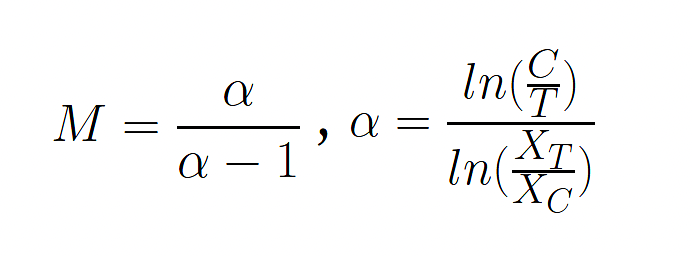
M is the multiplier of a given variable in a given year (subscript omitted); C is the number of observations above the lower cutoff (we use the 80th percentile); T is the topcoding threshold; and X_C and X_T are the lower cutoff and topcode threshold values, respectively.

As Armour and others warn, that method may produce unreasonable estimates if the topcoded variables are not Pareto‐​distributed over the relevant range. The shape parameter α is also highly sensitive to the threshold values because its estimation relies on only two distribution points. When we applied this method to the CPS variables, we found the estimated multipliers to be unreasonable in most years. Using income as an example, the multiplier M takes a believable value of 2.7 in 1994 but explodes to 28.7 in 2005 before fluctuating wildly and gradually dipping down to 1.1 in 2018. When exceptions to handle unreasonable multipliers are coded in, the statistical moments for all topcoded variables are not substantially different from the original methodology of simply assuming a multiple of 2. Justifying using such a volatile method paired with ad hoc adjustments is difficult, so we stuck with the original methodology for handling censored variables and multiplied topcoded values by 2.

The second change we attempted was to include a separate net fiscal cost estimate for illegal immigrants, but we were unable to implement it due to small sample sizes in the CPS. We attempted to locate them in the 1994–2018 CPS sample by using a residual methodology developed by Christian Gunadi, an economist at the University of California, San Diego, who imputed legal immigrant status and identified those remaining as illegal immigrants.⁸⁸ According to Gunadi’s method, people are counted as legal immigrants if they meet any of the following criteria, as recorded in the 2019 ACS: The immigrant arrived after 1980; is a U.S. citizen; received welfare benefits, such as Social Security, Supplemental Security Income, Medicaid, Medicare, or military insurance; served in the Armed Forces; worked for the government; resided in public housing or received rental subsidies or was the spouse of someone who resided in public housing or received rental subsidies; was born in Cuba and had a spouse who was a legal immigrant or U.S. citizen; or had occupational licenses. We omitted the occupational licensing criteria because of changes in the reporting in this variable in post‐​2017 census data, but that omission makes little difference to the final numbers.

Gunadi’s method works well for the larger ACS, but it identifies only 72,478 illegal immigrants in the CPS from 1994–2018. Because individuals can and do appear in multiple years in the CPS, the number of unique illegal immigrant individuals is even lower, at 61,652. As a result, many age and education groups have almost no illegal immigrant representation in the CPS sample, making it infeasible to obtain accurate fiscal profiles that are as granular and representative as the other profiles used in this model (see Table 24). Reduced illegal immigrant ineligibility for most benefits in this model means that the net fiscal impact of illegal immigrants would almost certainly be more positive than that of legal immigrants at the same age and education level, but we were unable to verify that because of the small sample sizes.

This section presents the estimated net fiscal impacts from the Cato Model. Table 25 reports subpopulation size for each generation, per capita receipts and outlays, and net fiscal impacts under Scenario 5 for each generation for different levels of government in 1994, 2013, and 2018 using the Cato Model. If the ratio of receipts to outlays is greater than 1, that subpopulation pays more in taxes than it receives in benefits. Table 25 corresponds to the earlier Table 2 and updates the NAS results for 2018, with additional columns reporting the results for the second and third‐​plus generations combined. The combined group is a good comparison to first‐​generation immigrants because there is no reason why second‐ and third‐​plus‐​generation individuals should be considered separately when comparing immigrants with native‐​born Americans. Figure 27 shows the annual net fiscal impact of each generation over time.

Allocating U.S.-born dependents of immigrants to the second generation greatly improves the net fiscal impact of the first generation because many of the outlays associated with raising children, including public education, have now been allocated to the native‐​born groups. The receipts‐​to‐​outlay ratio for the first generation is greater than 1 in every level of government and in total, meaning that the first generation pays more in taxes than it consumes in benefits, according to the methods followed for Table 25. To put their impact in perspective, in 2018, the average per capita fiscal contribution of first‐​generation immigrants was $16,207, whereas the average drain was $11,361, resulting in a net positive fiscal impact of $4,846 per immigrant in 2012 dollars. Multiplied by the number of immigrants present in 2018 (45.4 million), this amount results in a cumulative net fiscal impact of $220 billion. Adjusted for inflation, that number is 1.2 percent of the U.S. GDP in 2018 ($18.7 trillion in 2012 dollars) and 3.7 percent of all 2018 government spending ($6.031 trillion in 2012 dollars). The former figure is roughly in line with the Organisation for Economic Co‐​operation and Development’s (OECD) 2006–2018 estimates, which are 1 percent for the United States and between plus or minus 1 percent for most OECD countries.⁸⁹

Allocating the fiscal costs and benefits of the U.S.-born children of immigrants to the second generation dramatically improved the first generation’s impact on state/​local governments in recent years because those levels of government supply most public education. The second generation’s fiscal impacts have been revised significantly downward because the costs of U.S.-born dependents of immigrants now fall entirely on the second generation. However, the net fiscal impact for all native‐​born Americans is only revised slightly downward in Table 25, as the U.S.-born children of the first generation are a relatively small group compared with other native‐​born groups.

Although immigrants’ net fiscal impact at the federal level has worsened over time, it has improved at the state level, resulting in a net improvement from 1994–2018. The opposite is true for the second and third‐​plus generations, who have worse net fiscal impacts at the state level in more recent years.

Table 26 presents the same results as above but for all fiscal scenarios and for 2018 only. Under all scenarios, first‐​generation immigrants have a higher receipts‐​to‐​outlays ratio than that of native‐​born Americans. This finding is especially the case in Scenarios 5–8 because the total costs of public goods are attributed entirely to native‐​born Americans in those scenarios, meaning that immigrants naturally consume a comparatively small quantity of federal outlays. The only instance in which immigrants have a total net negative fiscal impact is under Scenario 3, but even in that case, their impact is less negative than that of the native‐​born groups.

We also replicated the NAS regressions comparing the fiscal impact of first‐​generation immigrants with native‐​born Americans when controlling for demographic characteristics (see Table 27). Note that because the baseline group now contains both second‐ and third‐​plus‐​generation natives, the coefficients are not directly comparable to those of the Updated Model presented in earlier sections. Despite that caveat, the coefficient signs of the Cato Model in Table 27 are identical to those of the NAS for Models 1, 2, 3, and 5. The only revision for which the sign has flipped is Model 4, in which all demographic characteristics are controlled for other than the number of dependents. In that case, immigrants go from having a net fiscal impact nearly identical to that of natives to having a slightly negative impact on the federal level.

This section presents the fiscal impact in NPV terms of individuals based on immigration status, education, and age using the methods we developed for the Cato Model. All changes made in the Cato Model apply to the underlying data used to calculate those NPVs except that the NPV method does not require allocating dependents by generation. A person’s NPV is based only on his individual fiscal flows and those of his potential descendants, calculated using probabilities for survival to certain ages, emigration, and fertility. The “descendants” component of the immigrant’s NPV therefore contains only potential people projected to exist in the future, not real observed people, meaning that immigrants do not have their dependents’ fiscal flows counted against them regardless of whether their dependents were born in the United States or abroad. Therefore, the change in dependent allocation does not apply to this section, but we broke out the NPV into the share attributable to the individual and the share attributable to his or her descendants so that readers can interpret NPVs differently if they so choose. In all other respects, this section follows the 2017 NAS methodology for calculating NPVs, with the appropriate Cato Model changes made to the underlying data (see Box 6 for a list of changes).

A person’s total fiscal NPV is highly dependent on his children’s projected level of education. In the Cato Model, educational attainment is only partially determined by parental education, and variability increases with each subsequent generation. That statement implies that even though first‐​generation immigrants are generally less educated than are native‐​born Americans, the second generation are more educated than their first‐​generation immigrant parents. Our method of predicting educational attainment for future generations uses the same independent variables as our method for imputing educational attainment for those younger than 25: parental education, immigrant birthplace, and parental birthplace. One key difference is that the random variability term gains a wider variance with each generation, indicating future uncertainty for education levels.

The results of those projections for the U.S.-born children of foreign‐​born parents and of native‐​born parents are in Tables 28, 29, and 30. Generally, the U.S.-born children of foreign‐​born parents have a higher likelihood of surpassing their parents’ education than the U.S.-born children of U.S.-born parents do, reflecting educational assimilation and the catchup effects for the children of less educated immigrants. For recent immigrants who are likely to be raising or about to have children (aged 20–30), their children are expected to improve their educational outcomes and pass that down to their children. Those results indicate that our projection methodology correctly captures the intuitive fact that the children of immigrants are likely to benefit from improved education relative to their parents.

Table 31 displays the NPV of fiscal flows in thousands of 2012 dollars, discounted at 3 percent, of an immigrant entering the country at 25 years old versus a 25‐​year‐​old native‐​born American. Recall that the results for immigrants have been adjusted to include formerly omitted capital income, which is adjusted by multiplying their taxes paid by between 1.6 and 1.9, depending on education level.⁹⁰ Lower‐​education cohorts benefit more from that adjustment relative to higher‐​education cohorts, but all immigrant groups experience a significant boost in the positivity of their fiscal impact. We separate results by education level, budget scenario, and fiscal assumptions. The results do not differ much by budget scenario, so we will focus on the “CBO long‐​term budget outlook” scenario.

Immigrant individuals are consistently fiscally positive, regardless of how we treat public goods under the various scenarios, whereas natives are a net fiscal drain if they are high school dropouts. Even though descendants are always a net fiscal burden in those cohorts, the total impact of the individual plus descendants is uniformly positive for immigrants and mostly positive for native‐​born Americans, although natives in lower‐​education cohorts struggle to cross this threshold, especially when public goods are included in benefits. For example, when public goods and interest payments are included, even natives with some college education have a fiscally negative impact because of their descendants. Lastly, immigrant descendants are consistently more fiscally negative than native‐​born descendants.

Table 32 shows net fiscal impacts for more‐​detailed cohorts (see Appendix B for tables showing the breakdown between capital income and state/​local and federal NPVs under different scenarios). The net fiscal impacts of descendants become negligible and the impact of individuals becomes increasingly negative when they immigrate to the United States at an older age (see Table 32). When comparing immigrants and native‐​born Americans with public goods, excluded under Scenario 5, we see that immigrants always have a more positive net fiscal impact than natives do, with the lone exception of newborn natives, who have been projected to obtain a graduate‐​level education. Even in that case, the gap is only $6,000 in the “No budget adjustments” scenario. Immigrants nearly always receive less in benefits than native‐​born Americans do and pay more in taxes when formerly omitted capital income is included.

Immigrants overall tend to have a much more positive fiscal impact than native‐​born Americans do in the post‐​2016 microdata, regardless of how public goods are treated (see Figure 28). Capital income accounts for most of this disparity. To present an alternative example without the tax from capital income, Figure 29 shows that immigrants still have a superior fiscal impact relative to native‐​born Americans. Immigrant emigration rates help explain their persistently better net fiscal impact. For instance, immigrants who arrive shortly after birth have an approximately 30 percent chance of emigrating from the United States by age 65. In those cases, immigrants are modeled as paying into the Social Security system for many of their working years and then emigrating before receiving retirement benefits, which reduces their consumption of government benefits relative to the taxes they pay.⁹¹

Aggregate differences are also largely accounted for by differing age profiles between the subpopulations. Compared with native‐​born Americans, immigrants are more concentrated in working‐​age cohorts. Recent arrivals are more likely to be younger and much less likely to be of retirement age. Combined with the aforementioned fact that the future children of immigrants will not be saddled with as severe an educational disadvantage (see Figures 28 and 29, which are for individuals plus descendants), immigrants, intuitively, would have more‐​positive future impacts on the fiscal balance. In general, including or excluding capital income affects the magnitude of the fiscal impact, but it does not change the sign. In addition, more‐​recent immigrants have a more positive net fiscal impact than do all immigrants and native‐​born Americans.

For the Updated Model, we examined how much of a reduction in welfare spending would be required to turn immigrant education cohorts with a negative net fiscal impact into fiscally neutral cohorts (Table 20). This subsection answers the same question using the Cato Model. Fiscal flows that are classified as welfare are unchanged (see Box 5). Table 34 shows the percentage reduction in welfare benefits that would make each cohort have a net fiscal impact of zero at the state/​local, federal, and total levels. Fiscally positive cohorts are recorded as “N/A.” For others, even reducing their welfare receipts to zero would not be enough, so the box says “>100%.”

Under the assumptions that include no public goods and exclude capital income, immigrants with only a high school education and natives with some college can become fiscally positive through reductions in welfare expenditures. Immigrants with a high school education would need a 48 percent reduction, and natives with some college would need a 60 percent reduction in welfare consumption to have a net fiscal impact of zero. When public goods are included in benefits for total state/​local and federal budgets, natives overall cannot be made fiscally neutral, but those with only a college degree can be neutral with a 20 percent reduction in welfare consumption.

When capital income is excluded from their overall fiscal impact, immigrants overall can be made neutral with a 50 percent reduction in welfare benefits even though the signs of any one immigrant cohort’s net fiscal impact cannot be changed in the “Public goods” scenario. At the federal level, immigrants can be fiscally positive at the federal level relatively easily even when including public goods, as immigrants require only a 4 percent reduction in welfare benefits to achieve that goal, whereas natives have an intractably negative net fiscal impact. Those results differ from those of the Updated Model. The Updated Model concurred with the Cato Model’s finding that immigrants overall can be made fiscally positive by slashing welfare spending but also implied that natives could have a zero net fiscal impact with a 20 percent reduction in welfare spending (see Table 20). When capital income is included, only immigrant high school dropouts and high school–only graduates are fiscally negative when public goods are included, and the latter group can be flipped with a 25 percent reduction in welfare spending (see Table 34).

This report analyzes how immigrants and native‐​born Americans affect the finances of the federal and state/​local governments in the United States in the recent past, currently, and projected into the future. We used two models to estimate the net fiscal impact of immigrants and native‐​born Americans. The first model we used is an updated version of the model used by the National Academies of Sciences, Engineering, and Medicine in 2017. Using the Updated Model with more‐​recent data and a small number of methodical changes made necessary due to limited data availability, we find that immigrants have a generally positive impact on federal government finances and a somewhat negative impact on the finances of state/​local governments, depending on the treatment of public goods. The ratio between receipts (taxes paid) and outlays (benefits received) has been historically lower for the third and second generations than for the first generation. For instance, under our preferred treatment of public goods, in which immigrants pay the marginal cost of those public goods (Scenario 5), the first generation had a fiscal ratio of 0.960, the second generation a ratio of 0.741, and the third a ratio of 0.747 in 2018 (see Table 2). Tax contributions from the third generation were the highest of all three immigrant groups, and federal outlays were the lowest for the first generation.

The second model is the Cato Model, developed for this paper and based on the 2017 NAS model, wherein we made several methodological changes to be consistent with more recent research on the fiscal impact of immigration. Those major changes are that the Cato Model adjusted NPVs for formerly omitted capital income, reallocated the fiscal impacts of U.S.-born dependents of immigrants to the second generation, used a different method for estimating the educational attainment for persons younger than 25, excluded the CBO’s deficit reduction scenario, removed the age limit on some federal programs, and used the PCE measure of inflation rather than the CPI. The Cato Model found that the first generation’s fiscal ratio was 1.427, the second generation’s was 0.452, and the third generation’s was 0.757 (Table 25). Per capita tax receipts were highest and outlays lowest for the first generation in 2018 (see Table 25). The decision to reallocate taxes and benefits to individuals who incurred them rather than to their parents decreased the tax contributions from the second generation because their population is primarily younger. Indeed, the second generation’s state/​local fiscal ratio was 0.362 in 2018 (see Table 25), the lowest of all measures in that year. The per capita tax contributions from first‐​generation immigrants are higher in the Cato Model because their U.S.-born children are regrouped into the second generation.

Historically, the fiscal impact of different population subgroups differs by characteristics other than nativity, namely age and education. Demographic groups whose population is concentrated in younger ages are a larger burden on state/​local government finances, mostly because of K–12 education spending. Populations with a larger elderly population are a comparatively larger burden on federal finances because of old‐​age health care and retirement benefits. Education is highly correlated with taxable income and lower welfare program usage. The patterns from different cost scenarios that treat public goods differently are similar under both the Cato Model and the Updated Model, with the most positive ratios for immigrant groups appearing under marginal cost scenarios and the lowest ratios under average cost scenarios.

Our net fiscal impact projections are different under the Cato Model compared with the Updated Model due to the inclusion of capital income, as recommended by Michael Clemens.⁹² Under the Updated Model, the total and federal net fiscal impact of immigrants is generally higher relative to natives for the young and less educated and lower relative to natives for the elderly and more highly educated. The state/​local net fiscal impacts are generally lower for immigrants of all education and age groups due to the different tax and spending structures on that level of government. State/​local governments bear most education costs and typically do not recoup those costs later in a person’s life through higher tax revenue, but the federal government does. The younger age distribution of immigrants and higher number of children per immigrant household help to explain that fiscal cost discrepancy. Federal benefits favor the elderly, so immigrants who are primarily working age receive fewer of those benefits. Immigrants are also less eligible than natives are for several federal means‐​tested welfare programs.

Our inclusion of capital income under the Cato Model results in immigrants having consistently more positive fiscal NPVs than those of native‐​born Americans, essentially resulting in a near doubling of their taxes paid depending on education level and leaving benefits untouched. The federal and state/​local dynamics are similar under both models, but the inclusion of taxes on capital paid by firms hiring newly arrived immigrants significantly changes the overall picture.

Projections of the future impacts are wide ranging. The Updated Model projects that immigrants will have a generally net positive impact on federal and state/​local budgets, with significant variation based on age of arrival and final education level. The Cato Model projects that immigration will have a large and consistent net positive impact on all government budgets. Results differ significantly depending on the treatment of public goods and are highly dependent on age and education demographics. If immigrants continue to arrive with higher levels of education and birth rates continue to fall, their relative fiscal contributions will continue to increase assuming there is no significant change in U.S. spending and tax policies. With some caveats, immigrants have a positive net impact on U.S. government budgets.

This appendix includes additional details on the methodology and data used in the projections of future impacts of immigrants for the Updated Model. All calculations and data sources are similar to those used by the NAS in 2017 unless otherwise specified. We first repeat and discuss the steps we took, in order, with information on data sources, and then we provide the data sources and assumptions used in estimating each tax and benefit variable. Note that most variable names are identical to the ones appearing in the 2017 NAS report.

Data for the tax and benefit flows come primarily from March extracts of the Current Population Survey (CPS) Annual Social and Economic Supplement. Our sample is restricted to 1994–2018 because interviewees were not asked for their citizenship status before 1994, and retirement income data (variable names SRCRETI1 and SCRETI2) are not available in more recent samples. Our sample provides 4,634,775 observations for analysis.

We created separate flows for three immigration groups with the five education levels defined in the Methodology section, which are smoothed using 3‑year samples so that aggregates on the year 1995 are the average of 1994–1996, the averages in 1996 are the average of 1995–1997, and so on. The household‐​level variables in the CPS supplement are allocated among household members according to the assumptions in the variable list in Table A2. Other goods are allocated equally to individuals in a particular group, such as refugee aid to immigrants and public expenditures to all individuals in the sample.

As explained in the historical methodology discussion, additional sources are used for the profiles where the CPS lacks data. For the profiles, those data include state per‐​pupil current spending from the Census Bureau’s Annual Survey of School System Finances; per‐​enrollee Medicare and Medicaid expenditures by age group and gender from the National Health Expenditure Accounts’ (NHEA) age and gender estimates; American Community Survey (ACS) samples on institutionalization for the available years 1980, 1990, and 2000–2018; the Census Bureau’s annual estimates of resident population; and three sources of aggregate spending controls.

Specifically, per‐​pupil current spending is published in a summary table titled “Per Pupil Current Spending (PPCS) Amounts and 1‑Year Percentage Changes for PPCS of Public Elementary‐​Secondary School Systems: US and State.” State‐​level per‐​pupil public education expenditures for the years 1994–2018 are reformatted to be a percentage of the reported total U.S. expenditures and reidentified by state Federal Information Processing Standards codes to be consistent with the CPS state identifiers. The data are then used to weigh total state/​local expenditures and are assigned in concurrence with school enrollment. Elementary and middle school students (ages 5–14) are assumed to have 100 percent enrollment. For high school students (CPS variable SCHLCOLL == 1 or SCHLCOLL == 2), a half weight is applied to those enrolled half‐​time. For elementary or junior high students (5‑to‐​14‐​year‐​olds), 100 percent enrollment is assumed.

Per‐​enrollee Medicare and Medicaid expenditures, by age group and gender, are from the NHEA age and gender estimates. The available NHEA data improve our health care estimates relative to the 2017 NAS report. The NHEA only recently began publishing per‐​enrollee expenditures, and the 2017 NAS report only had access to total per capita national expenditures, including Medicare, Medicaid, and other sources. The profile of Medicare and Medicaid expenditures is very different. Medicare consumption is highest at older ages, whereas Medicaid consumption is highest at younger ages. We used the average age and gender distribution for individuals who are enrolled in Medicare (HIMCARELY == 2) and Medicaid (HIMCAIDLY == 2) to allocate aggregate Medicare and Medicaid expenditures reported by the Centers for Medicare & Medicaid Services.

For the institutionalized population, we used Integrated Public Use Microdata Series ACS samples for the available years 1980, 1990, and 2000–2019 and interpolated for years without a sample. Individuals are separated into two groups depending on their immigration status. A person is defined as institutionalized if they live in group quarters (GQ == 3). Because the ACS does not ask individuals for their parents’ birthplace, second and third generations are not distinguishable in the data. The proportion institutionalized is thus assumed to be the same for both second and third generations, following the NAS’s 2017 approach. Additional assumptions made relating to the institutionalized population are summarized in Table A1.

CPS population reports for our sample 1994–2018 are adjusted to the mid‐​year total resident population using the Census Bureau’s Annual Estimates of the Resident Population for the United States. Those data are published between each census and only cover the intercensal period. When estimates overlap in 2000 and 2010, the most recent estimate is used. Data for the 1994–2000 estimates are the mid‐​year population estimates from the 1990s national tables.

Reports of aggregate receipts and payments come from three sources: the Bureau of Economic Analysis, the Office of Management and Budget, and the Centers for Medicare & Medicaid Services. From the Bureau of Economic Analysis’s National Income and Product Accounts, we obtain government outlays and receipts, domestic product and income, and additional details on pensions and retirement provisions; specifically, those data are in Tables 2.1, 3.1–3.6, 2.4.5, 3.8, 3.12, 3.14, 3.16, and 7.23–7.24. From the Office of Management and Budget’s historical tables, we used Table 2.1 (receipts by source of funds), 3.2 (outlays by function), and 12.3 (outlays for grants to state/​local governments). From the Centers for Medicare & Medicaid Services, we obtained hospital insurance and supplementary medical insurance expenditures from the annual Medicare Trustees Report and national health expenditures by type of service and source of funds from the National Health Expenditure Historical Data releases. Those data were used to adjust the totals provided by the CPS and to allocate public goods and other expenditures where necessary (see the variable list in Table A2).

We followed the NAS’s 2017 approach and assumed that individuals 25 years old or older in our sample have completed their education. We estimated the predicted future education of those younger than 25 by using a regression that predicts children’s education on the basis of their parents’ level of education.⁹³

From CPS samples from 1994 to 1999, we find a group of parents at least 25 years old who have at least one coresident child between ages 10 and 16 in the household. Neither of the parents can be a stepparent, and the parent linkages are restricted to the first mothers and fathers (MOMLOC and POPLOC), which excludes the partners of nonheterosexual family relationships. Those exclusions are necessary because the birthplaces of second mothers (MOMLOC2) and second fathers (POPLOC2) are not provided. Later updates to this model may have access to more complete data. For first‐​generation children, both they and their parents are identified as having been born outside the United States. Second‐​generation children are identified as having been born in the United States, with parents born abroad. Foreign‐​born children are identified as having been born in the same non‑U.S. region as their parents. We then use CPS samples from 2010–2018 to identify children aged 25–31 who fit the same criteria, giving us 10 paired child‐​parent linkages for the regressions. Even with four more linkages available, our regressions provided nearly identical results to the NAS 2017 results, which speaks to the strength of their estimates.

Ages 10–16 are used to maximize the sample size while ensuring that they are young enough to be living with their parents in the starting year and old enough to have mostly completed their education 15 years later. We considered using age 30 as a more conservative estimate to account for individuals pursuing higher degrees, but that cap reduced the sample available for the regressions too much to be worthwhile. To allow for greater granularity in our estimates, we then expanded the five education categories for the regressions and recoded the education groups into the five categories after estimation.

Parent‐​child groups are separated by birthplace region, which are the United States, Mexico, Central America (excluding Mexico), South America, Canada, Europe, Africa, East Asia, Southeast Asia, and Other Asia (including Eurasia, Central Asia, and Oceania). Then, for each region, the average education levels of children and parents were constructed and used to create four regressions. For the first generation, we constructed two regressions, separating out parental birth regions. One group includes children and parents born in Mexico, Central America, and South America. The other group includes all Europe and Asia regions. Canada and Africa were excluded because of low observation numbers. Members of the second‐​generation were not separated out by parental birth region.

For the Updated Model, the education regressions were applied to individuals younger than 25 observed in 2015–2018 to estimate future education attainments for the projected profiles. For the 1994–2018 sample, individuals younger than 25 were assigned their parent’s level of education (an average if the child has more than one coresident parent). The education of the child’s parent was used as the dependent variable to apply the regressions. For individuals with no coresident parents, the average educational attainment of the parents in the corresponding birthplace group 10 years prior was used, when the individual was more likely to be living with a parent. This imputation was necessary because the individual would be more likely to be living with parents 10 years before. Anyone else still without a parent in the household was assigned the householder education level for the regressions. Random error terms were applied to maintain variability in the education distributions. For the Cato Model, the education regressions were also applied to the individuals from birth to age 25 in the CPS 1994–2018 samples.

Thirty‐​year projections of tax and benefits were created for three budget scenarios: “CBO’s long‐​term budget outlook,” “CBO’s long‐​term budget outlook with deficit reduction,” and “No budget adjustments,” in which everything grows at the rate of total factor productivity growth, 1.1 percent.

Projections for 2021–2051 Scenarios 1 and 2 come from the supplementary files of the CBO’s 2021 Long-Term Budget Outlook. Expenditures by source are provided by “Table 1. Summary Extended Baseline” from the March 2021 budget supplement. Economic projections are provided by “Annual Values for Economic Variables That Underlie CBO’s Extended Baseline” and “Table 3. Economic Projections (Annual)” from the March 2021 economic supplement. Revenues are in the data underlying Figure 4 of the report. Data for years 2017, 2018, 2019, and 2020 are provided by the February 2021 historical report. Each variable is expressed as a percentage change from base year 2017 for the projections. State/​local flows were assumed to increase at the same rate as national GDP in the CBO baseline projection and the CBO budget reduction scenario, following the NAS 2017 methodology.

Per capita taxes and benefits for the “No budget adjustments” scenario in the 2017 profiles are increased at a rate of 1.1 percent each year, the rate of total factor productivity growth, in line with the CBO baseline projection.⁹⁴ This rate is greater than the NAS 2017 one that used a 1 percent assumed productivity growth rate based on earlier CBO baseline projections. For the other scenarios using CBO projections, the approach is different depending on whether the variable is considered in an average‐​cost or a marginal‐​cost case. For the flows that are identical for all age groups—that is, average cost—the method is the same as with the “No budget adjustments” scenario. Each group’s taxes and benefits reported in 2017 were increased at the rate from the CBO projections, including congestible public goods that include public expenditures. But for variables assigned on a marginal‐​cost basis, the native born are assigned a per capita amount that covers the aggregate amount estimated by the CBO, so the increase may be higher as the population is smaller.

For the flows that are not equivalent for all age groups, such as Social Security and public education, we used a population age distribution structure from the Census Bureau’s 2017 age and immigration population estimates (see Tables 9 and 10). Growth rates for each age group were applied separately to the first, second, and third‐​plus generations observed in the CPS sample. The second generation was assumed to grow at the same rate as the third‐​plus generation because the Census Bureau does not distinguish between the two. Changes in the number of people of a particular age were used to estimate the growth in variables sensitive to population changes.

Projecting the fiscal impacts of each individual and his descendants requires three key demographic estimates. Survivorship refers to the probability of an individual surviving in each successive year depending on age. Emigration probabilities were applied to the first generation to estimate the number of people leaving the sample. Again, following the NAS, this report assumes that children of immigrants younger than 20 emigrate with their parents, for both first and second generations. The number of descendants was estimated using age‐​specific fertility rates separated by generation and race.

Data on the number of individuals expected to survive to each age are given by the National Vital Statistics Reports 2018 Life Tables. Survival probabilities are given for each age (the range is from birth to 100 and older) and by racial group (non‐​Hispanic whites, non‐​Hispanic blacks, and Hispanics). Although long‐​term demographic projections are less important for a 30‐​year fiscal projection than for NAS’s 2017 75‐​year projections, the age and composition of a population are still important for accurate estimation.

We obtained data on emigration from the NAS 2017 report, and we did not alter them for our report. We also tested the Cato Model with higher emigration probabilities from a paper by Jennifer Van Hook and Weiwei Zhang, but that data resulted in unrealistically high emigration probabilities.⁹⁵ Surprisingly, it disadvantaged immigrants when calculating their net fiscal impact because they tended to emigrate in the middle of their most productive years, overwhelming the fiscally positive act of emigrating before retirement. The chances of young immigrants leaving the country by retirement age were upwards of 70 percent when using those numbers, so we deemed these probabilities too high and stuck with those used by the NAS.

The age‐​specific fertility rate measures the number of births per 1,000 women of childbearing age (15–50). Because fertility rates are higher for immigrants, we split women into first (variable BPL < 150 | CITIZEN == 3) and second‐​plus (variable BPL >= 150 & CITIZEN != 3) generations. Fertility rates are calculated using 5‑year age groups and further disaggregated by race. The racial categories are non‐​Hispanic whites (RACE == 1 & HISPAN == 0), non‐​Hispanic blacks (RACE == 2 & HISPAN == 0), non‐​Hispanic Asians (RACE >= 4 & RACE <= 6 & HISPAN == 0), and people of Hispanic origin (HISPAN != 0). Data come from the 5‑year Integrated Public Use Microdata Series American Current Population Survey 2019 sample. We used the age‐​specific fertility rate rather than other fertility measures because it is less affected by changes in the population age composition and is thus more useful for comparing subgroups over time.

After the tax and benefit profiles for each cohort were estimated, we applied the education of young persons to the 2017 profiles, and we had the projected profiles and relevant demographic data. The final step was to collapse the estimates for the 30 years down to a single comparable quantity. We weighed the projected per capita flows for each age, immigrant, and education group by their probability of survival and emigration for immigrants and constructed flows for their estimated children. Because our sample is 30 years, the impact of children is small.

For example, consider an immigrant arriving at age 52 with a college degree. The person is grouped into the profiles of immigrants of age 52 who have a college degree (education group 4) in 2017. For 2018, the group then becomes immigrants who are age 53 and have a college degree, they are given the estimated per capita profile accordingly, and so on until we reach 2051. For each year, the group is discounted by the probability that they survive to the next year. By 2051, this group will be 85, and the per capita flows will be greatly reduced to account for the higher death expectancy. This flow is then summed and discounted using a 3 percent discount rate.

An immigrant younger than 25 who arrived in 2017 (or a native‐​born American younger than 25 observed in the same year) will be assigned the tax and benefit profile using the parents’ education until he or she turns 25. At that point, education is estimated using the process detailed previously.

On the basis of the age‐​specific fertility rates, the probability of a newborn surviving, and a child not leaving with an immigrant parent, we estimated the number of expected children in each year. As with their parents, this group was multiplied by the taxes paid and benefits received as they progressed through the sample. If children reached childbearing age, this process was repeated for their expected children. For our sample, this group is understandably small. We do not expect to estimate the birth of many grandchildren over a 30‐​year time frame. Those children and grandchildren (if any) are included in the final summed and discounted net fiscal impact.

There is an inherent difficulty in counting which costs are attributed to immigrants and which costs should be attributed to their native‐​born second‐​generation children.⁹⁶ Although we believe that the allocation used in the Cato Model is correct, we understand that some may see this as giving an unfair advantage to first‐​generation immigrants. Appendix B contains the Cato Model results without changing the allocation of U.S.-born dependents of first‐​generation immigrants from the original NAS model. The tables below therefore correspond more closely to those in the NAS report.

The estimates in Table B1 reveal that the first generation and their dependent children still have a more positive net fiscal impact than that of either the second or third‐​plus generations, meaning that their tax payments are either greater than the value of the benefits they consume or closer than those of native‐​born individuals to covering the full costs. Furthermore, the first generation often shows a higher receipts‐​to‐​outlays ratio under the Cato Model (minus the change in dependent allocation) than it does under the Updated Model, but the difference is small in more recent years and sometimes reversed. The first generation and its dependents pay more taxes to the federal government than the value of federal benefits that they consume, but they consume more in state/​local benefits than they pay in state/​local taxes.

That pattern is reversed for the second and third‐​plus generations because their ratios are higher or the same at the state/​local level. That difference is mostly due to education costs, which are largely borne by state/​local governments. The federal and total fiscal ratio for the second generation has improved from 1994 to 2018, whereas it has been flat for the first and third‐​plus generations. Because the second generation is so young, moving into working‐​age years will continue to improve their federal and total fiscal impact. Even so, the overall ratio of 0.964 for first‐​generation immigrants and their dependents is significantly higher than the 0.739 and 0.769 ratios for the second and third‐​plus generations, respectively.

Table B2 presents the same results as Table B1 but for all fiscal scenarios. In all scenarios that allocate costs to immigrants on a marginal basis, immigrants have a fiscal impact superior to that of native‐​born Americans. In all scenarios in which immigrants are assumed to pay the average cost of public goods, the opposite is true. These results are nearly identical to those in Table 3 of the Updated Model.

As before, we replicated the regressions comparing the fiscal impact of first‐​generation immigrants and the second generation to the third‐​plus generation when controlling for certain demographic characteristics, this time without changing the allocation of dependents from the NAS model (Table B3). Although the signs of almost all coefficient estimates are the same as those in the NAS report and the Updated Model, the magnitudes often differ.

For Model 1, in which no controls were applied and the coefficients reflect the difference between group averages, the first generation still has a negative net fiscal impact compared with natives, but the impact has been revised from −$909 to −$913 at the federal level while remaining nearly identical at the state/​local level, resulting in a revision of the net impact from −$1,920 to −$1,921. That pattern persists in most specifications: The state/​local impact of the first and second generations relative to the third‐​plus generation remains nearly identical to the NAS results, as does the federal impact of the second generation. Meanwhile, the federal impact of the first generation retains its sign but is slightly revised in each model, but it has little effect on the net fiscal impact. Overall, our results for these regressions are very similar to those of the Updated Model.

Tables B4 and B5 show the NPVs for immigrants and native‐​born Americans under the Cato Model at the federal and state/​local levels, respectively, excluding public goods. Note that neither of these tables contains formerly omitted capital income because this flow is not exclusively received by either level of government. Table B8 shows the amount of capital income generated by immigrants for each age and education cohort and budget scenario. Table B6 is identical to Table 32 but includes public goods, interest payments, and capital income. Table B7 is identical to Table B4 but includes public goods and interest payments.

The authors wish to acknowledge the contributions of others to this white paper. Their helpful comments, suggestions, corrections, and edits improved this paper substantially. In alphabetical order, we acknowledge Zuha Afzal, David Bier, Bryan Caplan, Gretchen Donehower, Chris Edwards, Andrew Forrester, Chris Mackie, Jeff Miron, Aaron Steelman, Devin Thompson, Stan Veuger, and Danilo Zak. Any remaining mistakes are our own.

Nowrasteh, Alex, Sarah Eckhardt, and Michael Howard. “The Fiscal Impact of Immigration in the United States,” White Paper, Cato Institute, Washington, DC, March 21, 2023.