The child support collection process in the United States has largely failed. According to a 2020 Census Bureau report, only 62 percent of the more than $30 billion in authorized support payments for 2017 were actually received. While nearly 70 percent of custodial parents received at least some payments, less than half got their full amounts. Furthermore, average amounts received declined between 1993 and 2017, despite the inflation that occurred over that period. These observations raise the question of what factors may have led to the disappointing outcomes.
An important concern for an effective child support administration is the balance between award amounts and the monetary costs of raising children. When award amounts exceed these costs, the resulting incentives turn child custody into a financial asset funded by the difference between award and cost amounts. In such circumstances, unfortunate consequences follow. Contesting parties can gain monetary benefits from enhanced custodial positions and so make greater efforts to secure improved outcomes whatever the interests of the children.
Even when actual custody is not at issue, the presence of this financial asset creates resentment by the support obligor because it is his or her payments that fund the asset. This resentment can poison relationships between parents and lead to missed payments. Overall, an effective child support system relies on the willingness of obligor parents to make their assessed payments, which is an outcome greatly enhanced when the required payment amounts reflect the actual monetary costs of raising children.
In the past, award amounts were set through a judicial process that sought to balance the needs and equities involved. That changed sharply with the Child Support Amendments of 1984 that required states to adopt advisory child support guidelines. The guidelines became “legally presumptive” four years later in the 1988 Amendments.
To enforce those requirements, federal spending supporting state welfare programs was conditioned on the creation of the child support guidelines. States also were required to review their guidelines at least every four years. No longer would judicial outcomes depend entirely on evidence presented in court and pertaining to individual circumstances, but instead outcomes would be affected by political decisions embodied in statewide regulations.
While states were free to develop their own guidelines, the statute required that “as part of the [quadrennial] review of a state’s guidelines, a state must now consider economic data on the cost of raising children.” In effect, states were obligated to develop an economic model through which to determine child-rearing costs. Guideline amounts and judicial awards would then depend on those presumed costs.
The discussion below reviews and evaluates the economic models employed to create the state guidelines mandated by this legislation. The importance of these models is critical because the same data source has been used to derive very different results. The uniformly accepted data source is the Consumer Expenditure Survey (CES) published annually by the US Census Bureau. As a 2017 US Department of Agriculture report observed, these “data are the most comprehensive source of information on household expenditures available at the national level” (USDA 2017, p.2). Whatever divergent conclusions were put forth on the costs of raising children, the underlying data were not responsible.
Economic Data and Models
That the economic data do not speak for themselves was immediately evident in the CES reports. The reports provide expenditures for the important categories of housing, food, and transportation for an entire household rather than for individual members. From the start, it was thereby evident that an economic model was needed at least to allocate expenditures among household members.
In the years prior to the legislative changes, Robert Williams, a leading proponent of the new legislation, had argued that the principal deficiency of the established procedures was “a shortfall in the adequacy of [child support] orders when compared with the true costs of rearing children as measured by economic studies” (Williams 1987, p. 282). He stated that average court-ordered support obligations provided only about one-fourth of average expenditures on children “as estimated in an authoritative study by Thomas Espenshade [that] he judged the best available economic estimates of average expenditures on children” (p. 283). With that accolade, Espenshade’s analysis became widely adopted.
Williams suggested that “the root of the problem of determining child costs is that most expenses related to child rearing are commingled with expenditures benefiting all household members, … [including specifically] food, housing, and transportation” (p. 287). Rather than seeing this commingling of outlays as a positive factor that limited the additional costs needed to rear children because most household outlays already would have been made, Williams accepted Espenshade’s judgment that a new methodology was needed to avoid the commingling problem.
Living Standards or Expenditures?
Espenshade’s work had emphasized the distinction between living standards and actual expenditures. He wrote that because various expenditures “are conceptually difficult to assign to particular family members,” one should reject that effort entirely and move in a new direction. Instead, one should “develop an index of a family’s material standard of living and then … apply this index to a comparison of living standards of families that may differ … in size and composition” (Espenshade 1984, p. 19). In other words, to measure child costs, one should not rely on data reflecting actual expenditures but instead determine comparative living standards as between households with and without children.
To this end, Espenshade proposed a simple index for living standards that would be “the percentage … of consumption expenditures devoted to food consumed at home” (p. 19). To explain his approach, he offered the example of a childless couple that had total consumption expenditures of $6,091 used to maintain a particular standard of living as reflected by their food consumption. Now if that same or a similar family plus two children required total expenditures of $12,220 to reach a standard of living that included the same level of per-person food consumption, the overall cost of the children would be given by the difference between the two total consumption amounts, or $6,129 (pp. 21–22). Only at this higher expenditure level, he suggested, would the same living standard be attained.
This methodological approach now underlies the efforts used in most states to determine child costs. However, rather than using an index of “food consumed at home” to represent overall living standards, the currently employed index is expenditures on “adult clothing.” What has not changed is the presumption that overall living standards can be determined by outlays on a single commodity, and that the same index can be used for households both with and without children. To be sure, some households will value adult clothing more strongly than others, and of course preferences for clothing may be quite different in households with and without children. But those realities were ignored by the need to find an available index.
From the start, objections were raised. In particular, the authors of the USDA Child Cost reports emphasized that the Espenshade approach and its successors
do not provide direct estimates of how much is spent on a child. They estimate how much money families with children must be compensated to bring the parents to the same utility level (as gauged by an equivalence scale) of couples without children. This is a different question than “how much do parents spend on children?” [Morgan and Lino 1999, p. 198, emphasis added.]
In short, the values derived from such models are not expenditures at all, but instead are imputed values designed to equalize living standards in families with and without children.
Income Equivalence Models
The Rothbarth model, resting on adult clothing to indicate living standards, is a direct successor of Espenshade. A striking feature of this model is that although it does not deal directly with actual expenditures on children, its proponents suggest the opposite. They commonly refer to it as providing “actual economic evidence on child rearing expenditures” (Venohr 2013, p. 332), even though it provides instead imputed values that roughly reflect declines in adult utility levels resulting from supporting children on existing incomes.
Income equivalence models presume that spending on children by households with particular income levels necessarily means spending less on the adults in the households. From this presumption, Espenshade’s successors argue that the economic cost of raising children can be measured by the adults’ utility forgone from the fewer purchases made on adult-only goods due specifically to their support of children. The costs of raising children determined from these models are thereby the hypothetical amounts required to compensate the household adults for the welfare forgone as represented by their lower expenditures on adult clothing.
Whatever logic may pertain to this position, various issues arise that limit its adequacy as a measure of child costs. First, consumer purchases of specific goods and services are made when their own imputed values of a particular item exceed the prices paid for them. The required compensation used to define child costs thereby includes not merely the monetary expenditures for the replacement item but also the utility surplus (which economists call consumer surplus) resulting from the purchase. Therefore, consumer expenditures on particular items (such as adult clothing) are a poor measure of relative consumer values.
Second, and equally important, income equivalence models require the use of simplified proxies to represent utility levels. While Espenshade used the share of food in the household budget for this purpose, the Rothbarth model employs expenditures on adult clothing. While both approaches to income equivalence measures can be implemented, they require major restrictions on household utility functions that are quite limiting, and which has been criticized as unacceptable representations of household utility (Browning 1992, Pollack and Wales 1979).
Finally, whatever generalized variable is used, the income equivalence method requires making utility judgments in two very different states of the world: households with and without children. To the extent the household preferences shift when children are included in a household, as seems apparent, this index cannot determine relative utility levels. Making such comparisons from expenditures on adult clothing requires the assumption that preferences for this item remain the same with children as without (what economists call state-independent utilities). And without this assumption, there is no logical basis for making welfare comparisons. On this point, there is considerable support in the economic literature that utility functions are largely state-dependent (Frech 1994, Finkelstein et al. 2009). The income equivalence method fails most fundamentally because it requires the assumption that households without children have the same preferences for particular goods as do those with children.
I am not the first to dispute the adequacy of these models. As Martin Browning wrote more than 30 years ago:
The Rothbarth method imputes the same welfare level to households that have the same level of consumption to some adult-only good. Once again, I find it is difficult to see why this commands any widespread attention… .Without further justification this is surely unacceptable. [Browning 1992.]
The Importance of Household
Collective Goods
Among the CES expenditure categories, only about 15 percent of aggregate expenditures are readily classified as between household members (Betson 2010, p. 9). In particular, the largest three expenditure classifications are the household collective goods of housing, food, and transportation, where available data pertain to the entire household. What that designation signifies is that its use by one member of a household does not detract from its use by others.
The most prominent household collective good is housing, which is often a household’s largest budgetary item. While adults in a household benefit directly from this item, their children do so as well, and often without any additional cost. Only when additional housing costs are required by the presence of children do the incremental housing outlays represent a component of child costs. In effect, to use common economic terminology, children can effectively “free ride” on the collective goods provided by their parents.
To be sure, there are many circumstances where household housing costs are increased by the presence of children; and to this extent, the greater outlays are included in child costs. Children’s housing costs are thus limited to the incremental expenditures made in the presence of children that would not have been made otherwise.
Admittedly, there can be circumstances where collective goods are subject to congestion issues. Suppose additional children are rapidly imposed on a small dwelling that had previously served a two-person household; in that case, the household adults could possibly see their utility reduced with more children. However, that effect is unlikely with one, two, or even three children, although it might well exist with more children.
On these matters, David Betson, a leading proponent of the Rothbarth model, writes:
The childless couple, even though they have the same total spending, will be “wealthier” than the parents with the children… .Had the parents been childless, they would have been better off because the consumption of all other goods (i.e., those consumed by both adults and children like housing) would not be “shared” with the child. [Betson 2011, pp. 135, 185.]
As acknowledged here, a fundamental premise of income equivalence models is that parents are worse off because they share their household collective goods with their children.
However, Betson adds, there is a further qualification for the model’s applicability:
[O]nly if the composite good (that shared by parents with their children such as housing) were a pure public good would the family be able to avoid a decline in their material standard of living compared to a childless couple. [Betson 2011, p. 183, emphasis added.]
When this condition is satisfied, as it is when “congestion” issues do not detract from parents’ utility gained from living with their children, Rothbarth estimates would overstate child costs.
Income equivalence models rest on the presumption that parents do not gain “utility” from the presence of their children, but instead suffer a “disutility” as they are “crowded out” from their enjoyment of household collective goods. In these models, children are tantamount to strangers and tenants whose presence is a cost rather than family members whose presence is a joy. Income equivalence models require that parents need be compensated for this disutility, and that this prospective compensation should be included in the cost of raising children.
Recent USDA Reports on
Expenditures on Children
Unlike the income equivalence models, the annual USDA child cost reports (discontinued in 2017) seek to measure actual household expenditures on children from data collected by the same Census Bureau surveys. In doing so, however, the USDA faced the same conundrum that Espenshade had encountered: important expenditure categories pertain to the entire household rather than to individual members. To assign shares of these outlays to children required various assumptions; and attesting to their arbitrary nature, these assumptions were sometimes revised.
Prior to 2008, the USDA estimated children’s housing expenditures on a per-capita basis by dividing reported outlays by the number of people in the household. For example, in comparing household expenditures of a childless two-person household to a household of two adults and two children, the adult housing costs would now be half that of their childless counterpart, while the children’s allocated share would now equal that of their parents. Not surprisingly, under those conditions the housing costs allocated to children were substantial and became the largest item in the USDA reported child costs.
The USDA ultimately revised its estimating approach for housing expenditures. The 2017 report states that with “the rationale that the presence of a child does not affect the number of kitchens or living rooms, but does affect the number of bedrooms,” the USDA reports would not make per-capita housing computations. Instead, a child’s housing costs would become limited to “the average cost of an additional bedroom” (Lino et al. 2017, p. 98). Implicit in the revised approach is the presumption that a comparable household without children would occupy a similar dwelling but with fewer bedrooms. That approach thereby imposes an arbitrary structure on housing costs.
The food outlays allocated to children were equally arbitrary. Rather than employ the available Census data on household outlays for food, they relied on USDA optimal food plans: “Data from the 2015 Food Plans … were used to calculate the shares of total household food expenses spent on children.” These plans “increased with the age of the child but with little variation by household income” (Lino et al. 2017, p. 7). As with housing, these values were thereby imputed rather than observed. Because the imputed amounts represent ideal food budgets, lower observed values would suggest that such ideal budgets were often not followed.
And finally, the USDA reports manipulated the observed data on household transportation expenses. After deducting 25 percent of those outlays as related to employment, the authors divide the remaining transportation “expenses among household members in equal proportions” (Lino et al. 2017, p. 8). The USDA authors again made arbitrary decisions based more on presumptions than evidence.
Measuring Incremental Outlays for Children
This section reviews an alternate model that compares expenditures in households with and without children for the expenditure categories used by the Census Bureau. Instead of seeking costs related to individuals, this approach measures the increased household costs resulting from including children among its members. It includes incremental outlays for both private goods (such as children’s clothing and childcare) and collective goods (such as housing, food, and transportation) in their contributions to overall child costs. Critically, this method applies an incremental cost model that does not set arbitrary criteria to divide outlays on collective goods among household members.
In this analysis, we estimate regression equations for each category of household expenditures where the derived coefficients report how much more is spent on average in households with one child, two children, and three or more children as compared to households without children. From these equations, we derive actual additional expenditures for each commodity classification. And unlike the prior two models, these findings rest directly on data reporting consumer expenditures.
Although the results obtained here are different from those published in the USDA reports, this analysis employs the same expenditure categories. We can therefore compare the results obtained from the two models. Of particular interest is the finding that the USDA children’s housing cost figures are much higher than those derived from incremental household housing expenditures. There is thus little indication in these data that most households increase their housing budgets to include the cost of an additional bedroom for their children, although surely some do so.
Similarly, regarding household transportation costs, there is no indication that such costs are much different in households with children than those without. For this reason, the observed transportation cost applicable to children is minimal except for households with teenagers.
To determine the total cost of raising children, this model aggregates the incremental expenditures for households with children across the available expenditure categories. Like the other models, health care costs are not included. Rather than estimating costs related to individuals, this approach measures increased household costs from including children among its members. The statistical details from this process are contained in Comanor at al. 2015, although the values employed have been updated to current prices.
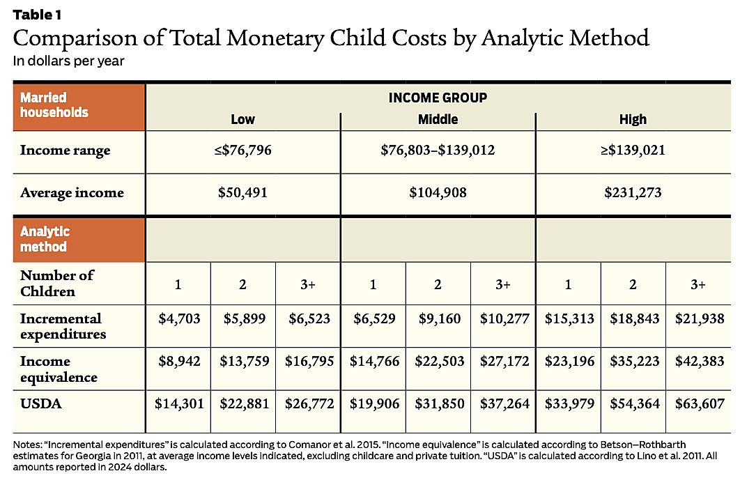
Table 1 compares the three models considered here. The most striking feature of these findings is the wide discrepancy from the other models. Indeed, the Income Equivalent values are sometimes more than twice those based on actual outlays. On this point, recall that Rothbarth values are not actual costs but instead presumed payments made to custodial parents for sharing their household collective goods with their children.
These results indicate that the arbitrary assumptions embodied in both the Income Equivalence and USDA models substantially increase the estimated child cost values as compared with actual measured amounts. In effect, both the Income Equivalence and USDA models impute substantially higher amounts than are reported expenditures.
Conclusion
The leading criticisms directed at this incremental outlays model do not deal with the method employed but instead at the results obtained (Venohr 2017, p. 4). However, finding variant results is not an adequate reason to prefer one model to another unless one is convinced from the start as to what are the appropriate conclusions.
What then becomes relevant is the distinction between economic costs and value. In principle, the former pertains to what one gives up for an outcome, while the latter refers to what one gains from the outcome. For the most part, these concepts track each other, but not always. And in the presence of household collective goods, they often diverge.
Unlike private goods, which are available for only a single person, collective goods are available to more than one person at the same time, and are those for which one person’s use does not substantially prevent another’s use and enjoyment. In particular, one person’s use of the family residence does not detract from another family member’s use. The critical point here is that a child’s welfare in the case of household collective goods is not measured by the costs attributable to him or her. In these circumstances, a child’s welfare may be great even when his or her costs are small.
This conclusion is important because guideline amounts exceeding the monetary costs of raising children can provide a substantial income transfer to the custodial parent and thereby represents disguised alimony. As such, the transfer can create resentment that leads to unpaid support obligations. The preferred policy is surely to provide child support awards that reflect the monetary costs incurred. For these reasons, during their next mandated quadrennial sessions, state agencies should adjust state guideline amounts to reflect more accurately the monetary cost of raising children.
Readings
- Betson, David, 2010, “Appendix A: Parental Expenditures on Children,” Review of Statewide Uniform Child Support Guidelines, Judicial Council of California, June.
- Browning, Martin, 1992, “Children and Household Economic Behavior,” Journal of Economic Literature 30(3): 1434–1475.
- Comanor, William S., Mark Sarro, and R. Mark Rogers, 2015, “The Monetary Costs of Raising Children,” Research in Law and Economics 27: 209–251.
- Edwards, R.D., 2010, “Optimal Portfolio Choice When Utility Depends on Health,” International Journal of Economic Theory 6(2): 205–225.
- Espenshade, Thomas J., 1984, Investing in Children: New Estimates of Parental Expenditures, Urban Institute Press.
- Finkelstein, Amy, Erzo Luttmer, and Matthew J. Notowidigdo, 2009, “Approaches to Estimating the Health State Dependence of the Utility Function,” American Economic Review, Papers & Proceedings 99(2): 116–121.
- Frech, H.E., 1994, “State-Dependent Utility and the Tort System as Insurance: Script Liability Versus Negligence,” International Review of Law and Economics 14(3): 261–271.
- Grall, Timothy, 2020, “Custodial Mothers and Fathers and Their Child Support, 2017,” US Census Bureau, May.
- Lino, Mark, Kevin Kuczynski, Nestor Rodriguez, and Tusa Rebecca Schap, 2017, “Expenditures on Children by Families, 2015,” US Department of Agriculture.
- Morgan, Laura W., and Mark Lino, 1999, “A Comparison of Child Support Awards Calculated Under States’ Child Support Guidelines with Expenditures on Children Calculated by the U.S. Department of Agriculture,” Family Law Quarterly 33(1): 191–218.
- Pollack, Robert A., and Terrance J. Wales, 1979, “Welfare Comparisons and Equivalence Scales,” American Economic Review 69(2): 2l6–22l.
- Rothbarth, Erwin, 1943, “Notes on a Method of Determining Equivalent Income for Families of Different Composition,” in C. Madge (ed.), War-Time Pattern of Spending and Saving, Cambridge University Press.
- Venohr, Jane C., 2013, “Child Support Guidelines and Guidelines Reviews: State Differences and Common Issues,” Family Law Quarterly 47(3): 327–352.
- Venohr, Jane C., 2017, “Review of Minnesota Child Support Guidelines, Economic Basis of Current Table and Potential Updates,” Center for Policy Research, March 31 (revised).
- Venohr, Jane C., and Robert G. Williams, 1999, “The Implication and Periodic Review of State Child Support Guidelines,” Family Law Quarterly 33(1): 7–37.
- Williams, Robert G., 1987, “Development of Guidelines for Child Support Orders, Part II,” Report to the US Office of Child Support Enforcement, May.
About the Author


This work is licensed under a Creative Commons Attribution-NonCommercial-ShareAlike 4.0 International License.