Environmental Costs of the Jones Act

This paper presents a detailed examination of the potential environmental gains that could be realized from reform or repeal of the law. It estimates that the environmental benefits accruing from the law’s repeal, through expanded use of waterborne transport as well as newer, more efficient vessels, would exceed $8 billion per year. Such gains are rarely estimated, if they are even considered.

To mitigate the adverse effects that transportation has on the environment, policymakers should acknowledge that the Jones Act encourages businesses to use less environmentally friendly forms of transport. Repeal of the Jones Act—or even a more limited set of reforms—would both promote economic growth and a cleaner environment.

Freight transport is an important service traded in largely competitive markets, but it gives rise to a variety of what economists call external costs. These costs are not borne by carriers or their customers, but by others who are not voluntary participants in the transaction. These costs are real: congestion, accidents, and noise all detract from total economic welfare. No carrier thinks about its marginal contribution to congestion, the increased chance of an accident, or the noise that one more truck creates as part of a consideration of whether or not to move another load of freight.

Environmental costs are an important class of external costs: air emissions, water contamination, and degradation of land resources are important examples of external environmental costs. The magnitude of these environmental spillovers is a function of the amount of freight transport and the choice of mode—truck, rail, air, or water—because they each have different environmental effects. Changing marine cabotage policy (“cabotage” refers to transportation between two places in the same country by a transport operator from another country) has the potential to change freight transport choices, with implications for transport markets and their external costs. This paper focuses on the net change in environmental costs from potential changes in marine cabotage policy.

Freight transportation is essential for the modern economy. We have grown accustomed to delivered consumer products, and industry has reengineered supply chains to minimize inventory costs and avoid costly delays. Transportation services account for a steady 3 percent of gross domestic product year after year, although waterborne transport—at less than 3 percent of total transportation value-added—is only a sliver of that.

As shown in Figure 1, most freight transportation moves by truck and rail, which account for more than two‐​thirds of the total ton‐​miles of freight movement. The third‐​largest mode is pipeline, which is particularly cost‐​effective for moving the petroleum and natural gas that the United States is producing in increasing quantities. Water transport includes ocean­going and inland waterway traffic (some of which is on the Great Lakes). Despite the physical advantages of buoyancy, which reduces the amount of energy required to move cargo a given distance, water transport accounts for only about 7 percent of the total freight movement trips.¹ Moreover, about 40 percent of the U.S. population lives along the coasts or Great Lakes, which underscores how underutilized water transportation may be.

With its heavy reliance on trucks, the United States has a much different freight transport network than other countries that are members of the Organisation for Economic Co‐​operation and Development (OECD). There are a number of reasons for this. Rail is the dominant freight mode throughout the OECD. After decades of regulation, the U.S. railroad industry has stabilized with fewer, larger railroads and lower rates. Physical endowments matter as much as policy in the nature of transport networks. No matter the enticement, Switzerland is unlikely to have much coastal waterway traffic, but Japan is likely to have a lot. The United States is mostly a continental market with a handful of isolated outposts—including Alaska, Hawaii, and Puerto Rico—that must rely heavily on marine transport. Short‐​term fluctuations in economic activity and fuel prices can affect demand for alternative transport modes, but long‐​term factors have an important influence. There is substantial path dependence in transport modes because of physical factors and long‐​term infrastructure investments.

Despite its ample water resources, U.S. water transport is restricted by the requirements of Section 27 of the Merchant Marine Act of 1920, commonly known as the Jones Act. The Jones Act requires that domestic waterborne transport of freight be conducted on vessels that are U.S.-built, owned, registered, and crewed. Colin Grabow, Inu Manak, Daniel Ikenson,² and Rob Quartel,³ among many others, have documented the distortions created by this provision. The century since the Jones Act’s passage has witnessed a dramatic decline in maritime transport. In an apparent effort to promote U.S. shipbuilding and U.S. shipping, the law has unwittingly incentivized alternative modes of transport, which generate environmental externalities that could be reduced under a different policy environment. The relatively few beneficiaries from the Jones Act receive gains at the expense of millions of consumers who absorb higher shipping costs, while the act imposes a great expense to the local and global environment upon which billions of humans depend.

Environmental costs from freight transport are substantial. Plausible changes to the current set of rules governing freight transport could reduce costs from emission in excess of $8 billion per year. While that translates into a welfare gain of about 1 percent of GDP from transportation, it represents more than 50 percent of the total value‐​added by water transportation. Accounting for avoided envi­ronmental costs provides strong additional motivation for Jones Act reform, with the upper bound increasing estimated welfare gains by 2 to 10 times.

The transportation industry is among the top producers of environmental externalities, which are particularly high relative to the industry’s contributions to GDP. The Environmental Protection Agency estimates that 14 percent of 2010 greenhouse gas (GHG) emissions were generated by the global transportation sector, with nearly all (95 percent) of the emissions stemming from the use of petroleum as fuel. However, the contribution of transportation to total environmental costs varies substantially across different types of emissions and therefore, via different paths, affects human well‐​being. In 2016, transportation accounted for 28 percent of U.S. greenhouse gas emissions. All modes of transport accounted for 58 percent of carbon monoxide emissions in the United States in 2014. Transportation sources from all modes accounted for 60 percent of nitrogen oxides (NOx) and 25 percent of volatile organic compounds (VOCs) emissions. Each of these types of emissions has different physical effects, including dispersion and longevity that affect the economic value of changes in emission levels.⁴

While the transport sector is responsible for sizeable proportions of total emissions, it has substantially reduced emissions across a range of criteria air pollutants since federal air regulations were implemented in the early 1970s, as shown in Figure 2. The transport sector has been far more successful than the nontransport (mostly fixed) sector in reducing emissions of criteria air pollutants, as well as other types of emissions. Removing lead from gasoline helped to dramatically reduce airborne lead levels, for example, with an attendant decrease in lead levels measured in human blood.⁵

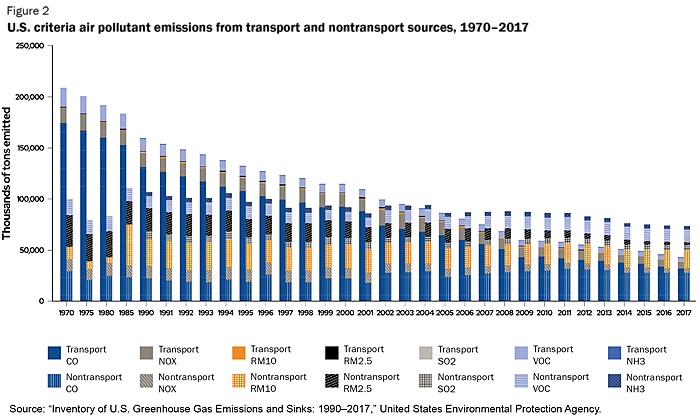
Figure 2 also shows how the criteria air pollutants emissions profile of transportation differs from other sources: carbon monoxide (CO) dominates transportation emissions, although NOx and VOCs also make large contributions. Relative to nontransport sources, emissions of particulate matter (PM), sulfur oxides (SOx), and ammonia (NH₃) are all both relatively and absolutely small. These differences between transport and other sources have not changed over time. While emissions intensity of transportation has fallen over recent decades, the compositional differences remain. This is important because integrated assessment modeling shows that the damages from emissions are highest for pollutants that are not prevalent from transport sources.⁶

Furthermore, Nicholas Z. Muller, Robert Mendelsohn, and William Nordhaus show that water transportation has very localized damages.⁷ Whereas highway and railroad emissions affect every county in the country, the damages from marine emissions are concentrated in coastal areas. And when criteria air pollutant emissions are released far from human populations, as is the case with marine transport to Alaska and Hawaii (which accounts for a significant amount of U.S. marine transport), the environmental costs are not as large. While that does not necessarily eliminate damages generated through other channels, the economic costs of local air pollutants depend on the location of emission. Greenhouse gases, in contrast, are global stock pollutants, which means their economic costs do not depend on the location of their emission.

While transportation has been relatively successful in reducing criteria air pollutant emissions, GHG emissions are a different story. Greenhouse gas emissions generated by the transportation sector increased by 20 percent between 1990 and 2016. Over that time, transport’s share of total U.S. greenhouse gas emissions increased from just under 24 percent to just over 27 percent. The good news is that relative to the overall transportation sector, maritime transport is relatively clean. Reallocating freight across modes has the potential to reduce GHG emissions.

Achieving such a shift would require some policy changes or other changes to encourage use of water transport, which has become less popular in the United States. In 1990, water transport of all types accounted for 6.7 percent of all transportation energy use in the United States. By 2016, water transport only accounted for 4 percent, even as transport energy use increased by 26 percent.⁸

Different transport modes generate different sets of environmental costs. Some ocean‐​going ships have traditionally burned residual fuel oil that is relatively high in sulfur, leading to much higher SOx emissions from that portion of the transport network, but a new low‐​sulfur standard mandated by the International Maritime Organization (IMO) limiting such emissions to 0.5 percent by weight (from a previous limit of 3.5 percent) took effect on January 1, 2020. Trucks are less energy efficient than ships, so they use more energy per ton‐​mile and generate more emissions, but U.S. trucks mostly burn low‐​sulfur diesel, so they have lower SOx emissions, all else being equal. As both ships and trucks move toward using natural gas as a fuel, the differences in their emissions profiles may disappear in the future. The coastal waters of the continental United States, Hawaii, and parts of Alaska are part of the Emissions Control Area, a designation that requires the use of low‐​sulfur marine fuels—with a standard even lower than the International Maritime Organization’s 2020 low‐​sulfur standard. As a result, expanding coastwise short‐​sea shipping within the Emissions Control Area will likely have less effect on SOx emissions than would a similar expansion using the global commercial fleet.

Table 1 compares the emissions profiles for different modes of freight transport, which reveals the importance of scale to waterborne freight emissions. The table includes a comparison of two different vessels, one large and one small, as measured by capacity. Shipping volume typically is measured in “twenty‐​foot equivalent units” (TEUs), which is the size of a standard shipping container with a maximum net cargo of 23.8 tons. The table highlights three basic findings. First, by requiring less energy to move a given amount of freight, ships can have much lower emissions than alternative transport modes. Second, this advantage depends heavily on the scale of waterborne transport—larger ships are cleaner than other modes, but the advantage declines for smaller ships. Third, waterborne freight has higher criteria air pollutant emissions.

Since the golden spike was driven to mark the completion of the first transcontinental railroad 150 years ago, much of the country has had a choice between transport modes. When the relative ease of a Pullman car beckoned, traveling from New York to San Francisco no longer meant a long and dangerous trip around Cape Horn or across Central America, both of which were journeys mostly by ship. Technological improve­ments have helped all transport modes, but the increased number of options—as well as costly mandates imposed by the Jones Act—bodes ill for the waterborne share of freight. Today, marine transport is primarily used where there are no substitutes, and the U.S. domestic oceangoing fleet has shrunk to a mere 99 ships. Using data from the Commodity Flow Survey, two‐​thirds of U.S. bluewater freight transport trips (excluding inland water­way and the Great Lakes) either originate or terminate in the noncontiguous states of Alaska and Hawaii, yet these trips carry only about 2 percent of the ton‐​mileage of U.S. water freight transport. Waterborne freight is concentrated in a handful of low‐​value, mostly time‐​insensitive, commodities. Nearly three‐​quarters of the waterborne ton‐​mileage of marine transport is in four classes of commodities: metallic ores, refined petroleum products, coal, and agricultural products.

By restricting the choice for domestic water­borne transport to qualified carriers, the Jones Act has raised costs for marine transport. Measuring these costs is a challenging empirical task. The first channel for impact is that the qualifications might directly raise production costs, either by requiring more expensive factors such as labor, or by specifying more costly performance standards, such as safety equipment. These changes must be measured relative to a historical transportation cost basis, so continuing technological improvement could lead to lower real costs and also to contemporaneous alternatives not subject to the same qualifications. Nonexclusive to the first, a second possibility is that substitute transport modes experience falling costs because of technological change or other policy measures. Third, the market structure in the domestic market may afford occupant firms short‐​term pricing power. Unless there are barriers to entry, in the long run firms cannot maintain market power. But the Jones Act does restrict entry to domestic firms and may act as an effective barrier to entry into the market. A fourth explanation is that short‐​term factors might reduce the long‐​term incentive for complementary investments, such as in ports, which then raise costs in the long run. The extent to which these factors amount to substantial and significant cost differences is an empirical question.

Surveys provide estimates of higher operating expenses for Jones Act–eligible vessels than for foreign‐​flagged vessels. The magnitude of the cost differential is contentious, but a variety of sources corroborate the intuition that the Jones Act contributes to higher costs for domestic shipping services. The U.S. Maritime Administration reported in 2011 an average operating cost for U.S.-flagged vessels that was 2.7 times higher than the foreign‐​flagged equivalent, mostly because of higher crew costs,⁹ while the Government Accountability Office noted in a 2018 report that “the relative cost of operating a U.S.-flag vessel compared to a foreign‐​flag vessel has increased in recent years.”¹⁰ Older estimates suggest that the cost differences have grown over time. The U.S. International Trade Commission (USITC) reported higher U.S. operating costs: from 110 percent for Aframax tankers¹¹ to 15 percent for 2,000-TEU containerships, which is consistent with earlier reports that found operating cost differentials of 52 percent for Aframax tankers and 13 percent for a 2,000-TEU containership, according to the USITC.¹² The OECD data provide a consistent picture: in 2018, the OECD Service Trade Restrictiveness Index rated the United States as 60 percent more restrictive than the average OECD country, which was about the same as the difference in 2014. Most of the barrier is attributable to Jones Act restric­tions on foreign entry.¹³

Existing information about cost differentials has been used to parameterize the USITC computable general equilibrium model that provides economic welfare estimates. In 2002, the USITC estimated that full liberalization of the Jones Act would increase U.S. economic welfare by $656 million (1999 U.S. dollars, equivalent to $1 billion in 2019).¹⁴ Removing only the domestic shipbuilding require­ment but keeping all other provisions of the Jones Act would deliver an increase of $261 million (1999 dollars, equivalent to $407 million in 2019) in economic welfare. Gary Clyde Hufbauer and Kimberly Ann Elliott found a similar topline figure using a different methodology, estimating that a full liberalization would increase U.S. economic welfare by $556 million (1990 dollars, equivalent to $1.1 billion in 2019).¹⁵ This gain is decom­posed into a $1.83 billion (1990 dollars, equivalent to $3.59 billion in 2019) gain for consumers of marine services and a $1.28 billion (1990 dollars, equivalent to $2.51 billion in 2019) loss for producers. Joseph Francois, Hugh M. Arce, Kenneth A. Reinart, and Joseph E. Flynn arrive at a higher estimate of $3 billion (1989 dollars, equivalent to $6.21 billion in 2019) in economic welfare cost, but add to the consensus that the Jones Act protects a relatively small number of jobs and firms at a broadly dispersed cost.¹⁶ None of these studies have attempted to enumerate the external costs, and so they potentially represent an underestimate of the burden of this law by measuring only direct cost differences.

The net effect of making waterborne transport relatively more expensive is that less freight moves by ship and boat than one might otherwise expect. In 2016, 4.2 percent of U.S. domestic freight tonnage was moved by water, compared to 65.7 percent by truck.¹⁷ Waterborne freight transport focused on low‐​value products, moving only 1.8 percent of total freight value. In 2015, 3.4 percent of domestic freight tonnage was moved by water, compared to 66.1 percent by truck.

Environmental costs are an important class of external costs associated with transport choices. Table 2 shows that in 2016, ships and other vessels accounted for only 0.9 percent of all freight GHG emissions, compared to more than 80 percent for trucks. The relative intensity of moving freight by different modes is shown in the final column of Table 2. Here water transport has a clear advantage: it is one‐​third lower than pipeline, 70 percent lower than rail, more than 80 percent lower than truck, and hundreds of times lower than air.¹⁸ So while water transport is not particularly competitive when environmental costs are excluded, taking GHG emissions into account makes water transport relatively more competitive among modes. How large this effect is relative to existing cost differences that drive current freight patterns, and how incorporating other types of environmental externalities affects the net balance, are all relevant to determining the environmental costs of the Jones Act.

Optimal transportation requires different considerations. Minimizing cost is one, but so too is timeliness, particularly in a world of just‐​in‐​time supply chain management. Envi­ronmental costs are another dimension to be considered. Given its importance to the modern economy, it is not surprising that transport choices have attracted considerable study, and the tradeoffs between modes are complex. Consider a hypothetical trip from Boston to Miami. Using the Geospatial Intermodal Freight Transport model (GIFT), the shortest‐​distance trip is one that relies heavily on ship, shaving about 150 miles (10 percent) off the shortest land route.¹⁹ That itinerary does not minimize the time spent traveling. While the ship delivers the cargo in a total travel time of 72 hours, the shortest‐​duration trip is about 24 hours with delivery by truck. Neither of these routes considers potential slowdowns, some of which might be predictable, such as traffic congestion or hours of service regulations for truckers, and some of which might not be predictable, such as weather.

Shipping rates take these differences into account. While ships may have lower unit costs than trucks, to the extent that they are slower, part of the cost savings is consumed by slower travel time. Bryan Comer et al. report delivery times at least four times longer by ship as compared to truck.²⁰ Conversely, a shipper might find it worthwhile to pay a premium for a truck to ensure direct delivery of a time‐​sensitive load. Shipping rates vary with the timeliness of delivery, and sometimes shippers are willing to pay more for speed; each day of transit time is equivalent to an ad valorem tariff between 0.6 and 2.1 percent.²¹ So a trip from Boston to Miami that takes three days instead of two might be expected to cost some 1.2 to 4.2 percent less. Naturally there are some products for which time is more valuable—fresh produce might be one example—and others that are less time‐​sensitive. The value of time is borne out in the lower costs of inventory that firms must hold with just‐​in‐​time delivery. Slower supply chains can be just‐​in‐​time as well, making the variance of delivery time more relevant to inventory costs. The fact that low‐​value products dominate water transport indicates that the time costs may be higher.

Returning to the GIFT model for travel between Boston and Miami, and considering the external costs of transport mode choices, can lead to still more variation. For example, to minimize carbon dioxide emissions on a per‐​TEU basis, ship transport is far preferred, in part because less than one‐​third of the energy inputs are needed to move the cargo by sea as opposed to land. But marine transport is not always the optimal transport mode. Other environmental criteria, including coarse particulate matter, SOx emissions, and NOx emissions, are minimized by truck transport. The net environmental cost savings depend on the value of these marginal changes in the composition of emissions between transportation modes.

The socially optimal transport choice is one that minimizes the total costs, including the monetary cost, the value of time, and external costs. A key question is whether reducing the amount of marine transportation decreases or increases the net environmental costs. Because marine transportation creates external environmental costs, it is true that reducing the amount of waterborne transport helps reduce those particular external costs. However, because freight that might otherwise be moved by boat or ship tends instead to be moved by some other means, the relative environmental cost for waterborne transport depends on the relative environmental costs across all transportation modes.

Mark Delucchi and Don McCubbin helpfully summarize a number of studies examining different types of external costs for both passenger and freight traffic. Compared to other transport modes, water transport lacks a comprehensive suite of studies, but where research has been conducted it has generally concluded that water transport has lower external costs than other transport modes.²² Table 3 summarizes those results, showing a range of economic damage estimates in cents per ton‐​mile that reflect differences across modes, in research methodologies, and different levels of scientific uncertainty about the magnitude of the external costs. For the external costs attributable to health effects from criteria air pollutants, the range of estimates is substantial but largely consistent across modes. Rail emerges as the lowest external cost mode in this regard, followed by water, air, and road. Consistent with Table 1 and Table 2, climate costs are lowest for water transport, thanks to lower fuel requirements due to buoyancy. Rail is second, followed by low‐​end road estimates. The range for road costs extends well behind the higher climate costs from air transport.

Rainer Friedrich and Emile Quinet provide a direct comparison between external cost estimates for water freight transport in the United States and Europe as part of a broader comparison between the transport systems.²³ The rank ordering across all modes is roughly the same between the United States and Europe. After converting units at current exchange rates, the comparison for water freight external costs attributable to air pollution indicates that the cost of those emissions is higher in the United States than in Europe (0.23–9.2 versus 0.11–1.4 dollars per ton‐​mile). The authors are careful to point out that the U.S. estimates include health effects but the European estimates do not, and that the European estimates reflect a much narrower range of scientific uncer­tainty thanks to a greater number of studies. A similar result holds for GHG emissions, with the U.S. estimates ranging higher than their European counterparts (0.0–0.67 versus 0.0–0.13 dollars per ton‐​mile). Together these results provide some weak evidence that the emissions profile of the U.S. water freight system generates slightly higher costs than the water freight system in Europe. Convergence between emissions costs from these two transport systems is possible: modernizing the U.S. fleet via repeal of the Jones Act or even its domestic‐​build requirement would be one step in that direction.

Expanding from just GHGs to criteria air pollutants, the environmental costs of freight transport become more nuanced. While water transport has lower external climate costs, it has higher criteria air pollutant emissions than other transport modes, notably rail. Taking these two types of emissions together, it is clear that water transport has lower external costs than air or truck. Rail and water have overlapping ranges of estimates, with rail being slightly lower. Comparing the United States to European countries reveals higher GHG emission costs in the United States. This is offset by slightly higher external costs from criteria air pollutant emissions, although the underlying methodologies are not comparable.

The Bureau of Transportation Statistics reports average revenues per ton‐​mile across transportation modes, which are also included in Table 2.²⁴ Under competitive conditions, these average revenues should be a good proxy for average costs. Consistently over time, water transport revenue has been between one‐​eighth or one‐​ninth of the revenue from trucks. In contrast, the cost difference between water and rail is much smaller, with barge rates as close as three‐​quarters of rail rates. The results are intuitive: planes cost more than trucks, which cost more than trains, which cost more than ships.

Internalizing external costs potentially changes the ordering of modes by costs. The high end of the range of external costs reported in Table 3 suggests that the environmental costs of water transport are potentially as high as the private costs. Truck transport is the only other mode that has as large a level of external costs. David Austin conducted a comprehensive study of external costs for truck and rail and found a lower ratio of external costs to market rates for trucks than is indicated by the figures shown in Table 2.²⁵ External costs have the least effect on air transport, in part because the market rates are already so high.

Forcing providers to pay external costs therefore has the largest relative effect on water transport and the smallest relative effect on air transport. However, when accounting for external costs, water transport has the lowest overall costs of any transport mode.

An important policy question is the degree to which today’s usage of different transport modes is attributable to the Jones Act and how much reflects intramodal competition. Estimating the environmental costs of the Jones Act requires three steps. The first is a comparison of the current situation and a counterfactual with a different cabotage regime. This paper uses existing estimates of the policy change. Second, a large literature evaluates the environmental costs of transportation outcomes across a range of measurable outcomes. Third, these two existing estimates are combined to project the effect of a policy change on environmental costs.

To calculate the environmental costs of the Jones Act, consider three counterfactuals. The first case imagines that the U.S. domestic fleet is upgraded to an international standard of emissions intensity, without any change in the volume of freight carried. The scenario reflects the relatively antiquated nature of the U.S. fleet, as compared to similar international fleets. In 2017, nearly one‐​third of all U.S.-flagged vessels were more than 25 years old—excluding the towboats and barges, the proportion was more than 53 percent.²⁶ Because modern vessels are likely to have lower external environmental costs as a function of technological progress, the Jones Act fleet’s modernization alone might offer scope for improvement.

The second case considers the effect of increasing maritime freight transport by 10 percent, displacing truck and rail transport in equal proportions. This counterfactual reallocates freight from truck and rail to maritime shipping. Hufbauer and Elliott provide some of the only quantitative estimates of reducing maritime cabotage barriers: they estimate a 22 percent price reduction as a result of complete repeal and an underlying supply elasticity of one.²⁷ The posited extensive effect is therefore something less than previous estimates of the effect of a full repeal of the act. These scenarios provide short‐​run estimates of cost savings, even though the physical transitions might take some time. The third case includes both the intensive and extensive effects. The scope of a liberalization, let alone its effects, are uncertain.

Table 4 summarizes the effect on environmental costs from freight transport under these three alternative counterfactuals. In the first case, upgrading the Jones Act fleet to lower‐​emissions vessels comparable to those found in Europe—purchases of which would become far cheaper after removal of the Jones Act’s domestic‐​build requirement—would avoid environmental costs mostly attributable to criteria air pollutant emissions. In part because of uncertainty about the magnitude of the environmental cost from these emissions, these avoided costs range from $118 million to $3.96 billion.

The second case offers a chance for more freight to move by ship by displacing truck and rail traffic. Such a displacement would be incentivized by waterborne freight transport cost reductions realized through Jones Act reform or repeal. The relative cleanliness of water transport compared to truck and rail comes into play at this point. This is reflected in the larger share of avoided costs of GHG emissions from switching freight to a more energy‐​efficient transport mode. In this case, the higher profile of water transport for criteria air pollutant emissions suggests that there could be a slight increase in environmental costs, mostly as relatively cleaner train traffic is replaced by the potentially most environmentally costly part of the U.S. fleet. However, the net avoided costs range higher than in the first case as more freight is reallocated to ships. This extensive change in water freight transport represents a real gain for the marine shipping sector.

The third case combines the first two cases, with waterborne transport becoming both more widespread and more environmentally friendly as older vessels are replaced with newer ones. The range of potential avoided costs in this scenario is from $109 million to $8.2 billion. To put the $8.2 billion figure into context, it is more than 50 percent of recent value‐​added from water transportation, or about 1 percent of the total transportation contribution to GDP. Given previous estimates of economic welfare gains from Jones Act reform that top out at $3 billion, the large estimated environmental benefits greatly strengthen the case for revisiting this law.

Changing the composition of the U.S. marine freight fleet to move more cargo raises a variety of other concerns that might be considered. Jones Act reform could deliver benefits indirectly by changing emissions profiles. A variety of other policies designed to provide an incentive to internalize external costs have been employed and discussed, and those policies could have a first‐​order effect on freight transport. The United States has relied on different mechanisms to control criteria air pollutant emissions, including technical standards that help explain the marked improvement in emissions intensity as shown in Figure 1. Because freight transport in general, and water transport in particular, are small relative to total environmental costs from transport, the sector was not focused on in the past. The exception to this is the Emission Control Area, which limits the sulfur content of marine fuels.

The current Jones Act–eligible fleet is disproportionately skewed toward tankers: 57 of 99 oceangoing vessels are tankers and they represent 80 percent of deadweight tonnage. One reason is the reliance on tankers to deliver oil from Alaska. In the short run, without a change in the fleet, the only way to increase the volume of freight transported by the Jones Act fleet is to use the existing stock of tankers. That means moving crude oil and refined products, which brings with it an increased risk of oil spills. While the Jones Act fleet is entirely comprised of double‐​hulled tankers, which have a lower risk of catastrophic spills, there is still a risk and an economic value attached to moving more oil and refined products in tankers.²⁸ In the event of a major spill in U.S. coastal waters, Jones Act waivers are needed to allow international fleets to help respond and remediate.

Oil and refined products’ disproportionate share of waterborne freight is a cautionary indication of the Jones Act’s effect. Because recent expansions in oil production have not been in Alaska where marine transport is required, the tradeoff has focused on pipelines versus rail.²⁹ Increasing utilization of the current fleet requires that increased bluewater freight be liquids. Bulk carriers are very limited, and other types of potentially useful ships, such as LNG [liquefied natural gas] tankers, do not exist under current build requirements.

Another important question is who stands to gain or lose from the environmental cost standpoint if the Jones Act were revised. In the event that a reform of the act resulted in a net shift of freight transport to marine and inland waterways, then local external costs might be felt by different groups of people. Broadly speaking, people near ports would likely be exposed to greater external costs, while those near highways or railroads would experience somewhat lower costs. To the extent that external costs are global rather than local, only the net change matters because local incidence is not an issue.

There are other external costs that might be alleviated by reform of the Jones Act. These include highway congestion, train derailments, and motor vehicle accidents. Further analysis of these external costs could further strengthen the case for Jones Act reform. There are also other potential environmental costs that could be accounted for, both directly and indirectly. Other direct costs are likely to be dominated by the public good nature of the air emissions.

There could also be further indirect effects embedded in supply chains. By limiting domestic shipment of time‐​insensitive bulk commodities such as scrap steel, the Jones Act unwittingly and unintentionally increases global emissions by diverting industry to foreign soil. The U.S. steel industry is among the cleanest in the world. When electric arc producers are unable to economically ship the scrap feedstock to their mills, foreign producers are only too happy to commission foreign‐​flagged vessels to export steel scrap to fuel their industry. The leading class of U.S. steel exports is scrap. Some steel smelted from U.S. scrap is reimported, further under­cutting the American steel industry. Local and global envi­ronments lose out on the trade. If affordable short‐​sea shipping could move scrap steel to steel minimills or even legacy producers, there would be a double dividend for marine carriers and the domestic steel industry.

Because GHG emissions are such an impor­tant factor in determining the environmental costs of waterborne shipping, the carbon price is a key consideration. The cost of carbon applies to all modes of transport, with water transport the least costly mode. Increasing the marginal cost of carbon emissions, either by assessing higher damages or limiting emissions, will increase the calculated environmental costs of the Jones Act. Reducing the social cost of carbon, as some in the United States have recently argued, will decrease the magnitude of environmental costs.

Changing the Jones Act offers the prospect of substantially reducing environmental costs created by freight transport. Using more marine transport would reduce the emissions from freight transport, especially for greenhouse gases. Criteria air pollutant emissions from water transport are slightly higher than for rail, but lower than for trucks. Both intensive and extensive changes to the prevailing regime could yield external environmental cost reductions of as much as $8 billion per year. These gains provide strong additional motivation for Jones Act reform. While previous studies have provided a range of economic welfare gains from easing the law’s restrictions, the environmental gains offer a substantial boost. Using the most conservative estimates of the gains from reform, the environmental benefits increase the net gains by 50 percent. Much larger gains are possible, increasing the benefits of reform by double or more.

Accounting for the external costs of transport services results in lower consumption. Various mechanisms exist to encourage decision­makers to internalize the costs, including taxing the activity in proportion to the marginal external costs. The change in the overall consumption of transport services is a function of the size of external costs and the elasticities of supply and demand for transport services. Allowing for multiple transport modes with different marginal external costs reallocates market share toward the mode with relatively lower marginal external costs. While the total amount of external cost will decrease, the amount attributable to the lower marginal cost mode will increase.

Accounting for the external costs of the Jones Act requires a second consideration: the Jones Act’s effect in the transport market. The top panel of Figure A1 represents the Jones Act as a supply shifter for the waterborne transport sector. Because waterborne transport is small relative to the total transport industry, and the Jones Act does not affect the supply of other modes of transport, the overall shift is smaller. Holding demand constant, the net effect is a reduction in overall transport from Q to Q′, and a corresponding private cost increase. The magnitude of these shifts depends on the price elasticity of demand and the aggre­gate supply elasticity. Under this specification the market share of waterborne transport decreases from Q_W/Q to Q′_W/Q′. This is a short‐​run change. In the long run, the elasticity of supply in the waterborne sector is likely to decrease because of barriers to entry and lower capital investment attributable to smaller quasi‐​rents.

The lower panel of Figure A1 shows the effect of the policy regime on external costs, without explicitly forcing carriers to internalize external costs. The shift from restricted supply S′_W to unrestricted S_W has three theoretical effects that ultimately lead to empirical questions. First, the increase in the amount of waterborne transport increases the total external costs from waterborne transport by area A. This increase in market share comes at the expense of nonwaterborne transport that has higher marginal external costs. The second theoretical effect is a decrease in external costs from nonwaterborne transport of A + B. The reduction of external costs from nonwaterborne transport (A + B) is partially offset by the increased external costs from waterborne transport A, implying a net reduction of external costs equal to area B. The third effect is an overall increase in transport, which increases external costs by area C. Combining these three effects, the net change in external costs from the policy change shifting SW is a reduction of area B — C.

The empirical magnitude of this change depends on a handful of parameters. The first shift depends on the marginal external costs of waterborne transport and the increase in traffic from the policy change, which depends on the size of the supply shift and the elasticity of supply for the sector. The displacement of higher‐​cost modes of transport depends on the difference in marginal external costs between waterborne and other transport. The third effect, the extensive increase in transport, depends on the elasticities of supply and demand for transport. In summary, supply elasticities for waterborne and total transport, a demand elasticity for transport, and the expected cost decrease of the policy change are the key parameters that are needed.

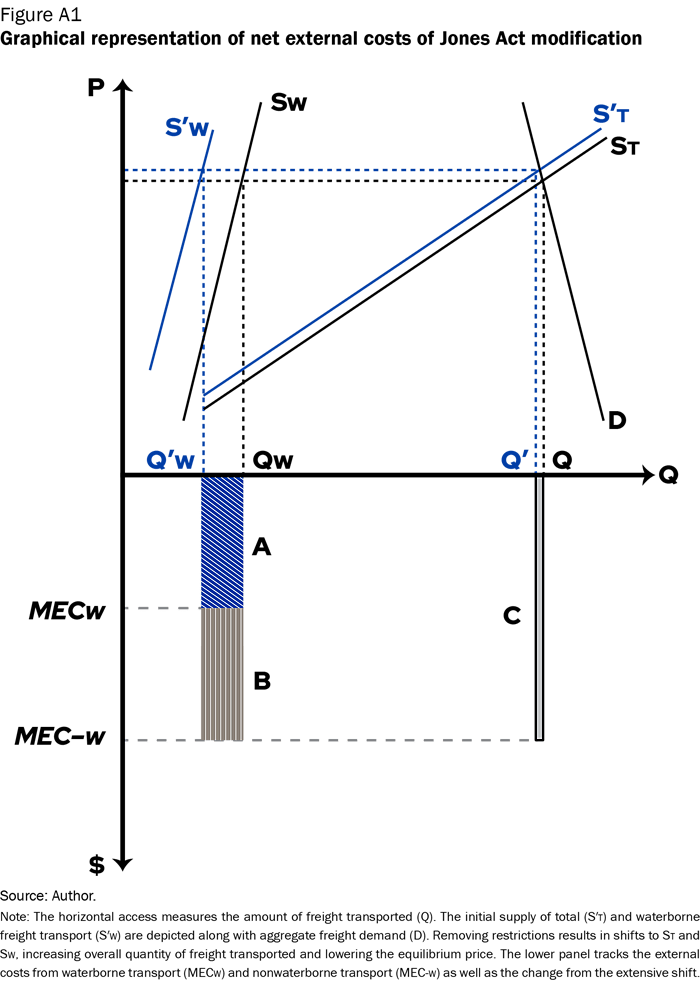
One final note deserves mention. The lower panel of Figure A1 represents the marginal external costs as constant over the relevant ranges. That need not be the case. It is possible, if not plausible, that marginal external costs could change in a way that alters the net gains of B from displacing other modes with waterborne transport. If

(holding the relationship at Q′_W constant), the policy change could increase marginal external costs by area

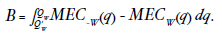
As an empirical matter, the marginal external costs are unlikely to change much over the relevant ranges from this policy change.

Fitzgerald, Timothy. “Environmental Costs of the Jones Act.” Policy Analysis No. 886, Cato Institute, Washington, DC, March 2, 2020. https://doi.org/10.36009/PA.886.