A previous article in this journal, “Optimal Tax Rates: A Review and Critique” (Reynolds 2019), analyzed such U.S. postwar ETI estimates that were being misconstrued as recommendations for a 73–83 percent optimal top tax rate for the federal income tax alone. I surveyed evidence and arguments suggesting that even if top tax rates designed to maximize short‐​term revenue might be “socially optimal” in some sense, such high marginal rates would not prove to be economically optimal in terms of the incentive effects on sources of longer‐​term expansion of the economy and the tax base. As Goolsbee (1999: 38) rightly emphasized, “The fact that efficiency costs rise with the square of the tax rate is likely to make the optimal rate well below the revenue maximizing rate.”

The early paper by Goolsbee included estimates of the ETI in the 1920s and 1930s. Together with another paper about the ETI during those years, by Romer and Romer (2014), the prewar studies came to nearly the same conclusion as their postwar counterparts did—namely, that hypothetical top tax rates of 74–83 percent could have maximized federal tax revenues during the Great Depression. Unlike Diamond and Saez (2011), however, the prewar studies excluded state and local taxes (which were much larger than federal taxes) and major new federal taxes on payrolls and sales added in 1932–37.

Romer and Romer (2014: 269) use an average of ETI estimates for federal income tax changes from 1918 to 1941 to conclude that “our estimated elasticity of 0.21 implies an optimal top marginal rate of 74 percent” (2014: 269). Yet their estimated elasticity is twice that high for 1932 (0.42) when the top marginal rate was raised from 25 percent to 63 percent. And their elasticity coefficients for major tax changes in 1934–38, they acknowledge, “cannot be estimated with any useful degree of precision” (2014: 266).

Goolsbee (1999: 36) compares 1931 and 1935 to judge how high‐​income taxpayers responded to much higher tax rates in 1932 (and higher still in 1934). He concludes the ETI at high incomes was so low that “if there were only one rate in the tax code, the revenue maximizing tax rate given the [low] elasticity estimated … [would be] 83 percent using the using 1931 to 1935 data.”

When discussing a smaller 1936 rate increase, confined to incomes above $50,000, Goolsbee concludes: “Technically, the revenue‐​maximizing [single tax] rate would be at the maximum of 100 percent using 1934–38 data, since the elasticity was negative” (ibid). A study of postwar data by Piketty, Saez, and Stantcheva (2014: 252) likewise theorized that “the optimal top tax rate … actually goes to 100 percent if the real supply‐​side elasticity is very small.” My review of that paper (Reynolds 2019: 250–54) found their estimated ETI and Pareto parameters to be far below consensus estimates for high incomes and inapplicable to untested tax rates of 83–100 percent. This review of similar prewar studies also finds their ETI estimates implausibly low and the alleged revenue‐​maximizing tax rates of 74–83 percent too high.

Romer and Romer (2014) are incorrect in claiming that tax responsiveness was low in the 1920s and 1930s, and Goolsbee is incorrect in making that same claim about just the 1930s. Their erroneous low response estimates lead them to conclude that high tax rates are a good thing. This study finds, instead, that high income taxpayers were very responsive to lower marginal tax rates in the 1920s and higher marginal tax rates in the 1930s.

I find that large reductions in marginal tax rates on incomes above $50,000 in the 1920s were always matched by large increases in the amount of high income reported and taxed. Large increases in marginal tax rates on incomes above $50,000 in the 1930s were almost always matched by large reductions in the amount of high income reported and taxed, with a brief exception connected with the 1937–38 recession, which is investigated in detail.

An earlier generation of economists found that raising tax rates on incomes, profits, and sales in the 1930s was inexcusably destructive. In 1956, MIT economist E. Cary Brown pointed to the “highly deflationary impact” of the Revenue Act of 1932, which

pushed up rates virtually across the board, but notably on the lower‐​and middle‐​income groups. The scope of the act was clearly the equivalent of major wartime enactments. Personal income tax exemptions were slashed, the normal‐​tax as well as surtax rates were sharply raised, and the earned‐​income credit equal to 25 per cent of taxes on low incomes was repealed [Brown 1956: 868–69].

In 1958, Arthur Burns wrote:

In 1966, Herbert Stein referred to President Hoover’s 1932 policies as “the desperate folly of raising taxes in a deep recession” (Stein 1966: 223). In contrast, Romer and Romer (2014) viewed their ETI estimates for 1932–38 as evidence that enormous tax increases in those years had no visible adverse effects on the Depression. To demonstrate the supposedly negligible impact of much higher income and excise taxes in 1932, they enumerate a few upbeat statistics about short‐​term business conditions. Meanwhile, Cole and Ohanian (1999) and Mulligan (2002) have been even more vocal in asserting that federal income and excise tax increases during 1932–36 share no responsibility for the depressing performance of the economy (and income tax receipts) from 1930 to 1940. The final sections of this article question the “taxes don’t matter” arguments and evidence of Romer and Romer, Cole and Ohanian, and Mulligan. Before doing so, however, we must first begin with a scenic detour of some new graphical evidence suggesting that most ETI estimates in Romer and Romer, and Goolsbee, are implausibly low, particularly for higher tax rates in 1932 and 1936.

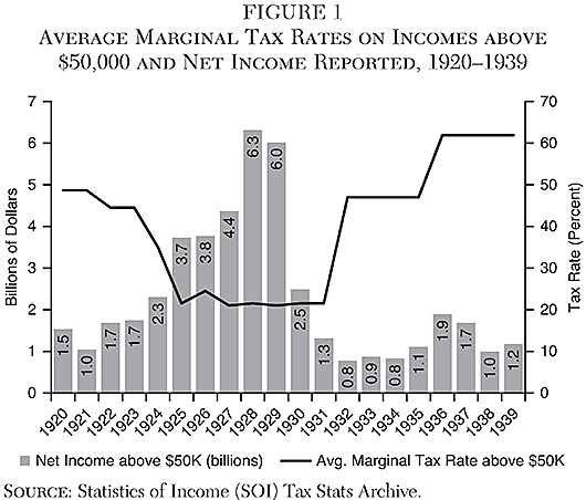
Figure 1 illustrates yearly connections between (1) changes in the average of all marginal tax rates applied to annual incomes above $50,000, and (2) the amount of net income, in billions of dollars, reported at incomes above $50,000. Taxable incomes of high‐​income taxpayers have grown rapidly when their marginal tax rates were low, and were flat or falling when their marginal tax rates were high. The only apparent exception was 1936–37 when taxable earnings above $50,000 briefly reached the equally unimpressive lows of 1922–23.

Romer and Romer (2014: 248, 252) define “high income” as the top 0.05 percent of income earners, which comprise “about 25,000 returns per year.” Taxpayers in that group and the incomes required to be included don’t remain constant from year to year. Indeed, “net income cutoffs for being in this group ranged from $25,400 in 1933 to $75,100 in 1928” (2014: 248). Consequently, defining high income as a percentage of income makes it a moving target for studying taxpayer response. Romer and Romer (2014) allocate marginal tax rates according to incomes on tax returns. But an income of $25,400 in 1933 faced only a 21 percent marginal rate in 1933—one-third of the top tax rate of 63 percent that year and even lower than the 23 percent marginal tax on $75,100 in 1928. Thus, we are unlikely to find a meaningful estimate of how high‐​income taxpayers react to high marginal tax rates by measuring how they reacted to marginal tax rates as low as 21 percent.

Figure 1 defines high income in a simpler way that is more transparently linked to tax rate schedules—namely, as net (taxable) income above $50,000—which, in 1935, included 10,680 tax returns and made up the top 0.33 percent of taxpayers (Tax Policy Center 2019b). That threshold combines the two highest of Goolsbee’s three high‐​income groups. It matches the definition of affluence in FDR’s 1936 tax law, which raised tax rates only on those earning over $50,000. Net income figures above $50,000 are added up from tax returns (SOI Tax Stats Archive). The graph is confined to 1920–39 to minimize possible distortions for 1918–19 caused by WWI and for 1940–41 by rearmament, though including those years would not make a great difference except for 1941.

The recession from January 1920 to July 1921 would have reduced high incomes regardless of tax policy. Yet the quest for a strong recovery from that recession was a major reason the average of various marginal tax rates on incomes of $50,000 or more (in Figure 1) was cut by more than half—from 48.7 percent in 1921 to 44.5 percent in 1922–23, to 35 percent in 1924, to 21.5 percent from 1925 to 1931.

Tax rates on net income below $10,000 were also reduced from 4–11 percent in 1921 to 1.5–5 percent from 1925 to 1931, and the personal exemption for couples was raised from $2,000 in 1920 to $3,500 from 1925 to 1931. Taxes paid by lower‐​income groups did fall. However, total individual tax receipts rose quickly—from $704 million in 1924 to nearly $1.2 billion in 1928. That is because the share of individual income tax paid by the over-$50,000 group nearly doubled in seven years—from 44.2 percent in 1921 to 51.8 percent in 1922, 69 percent in 1925, and 78.4 percent in 1928 (Frenze 1982). Moreover, the amount of revenue collected from high incomes above $50,000 nearly tripled at that time—rising from $318 million in 1921 to $507 million in 1925, and $909 million in 1928.

In Figure 1, the average marginal tax rate is an unweighted average of statutory tax brackets applying to all income groups reporting more than $50,000 of income. After President Hoover’s June 1932 tax increase (retroactive to January) the number of tax brackets above $50,000 quadrupled from 8 to 32, ranging from 31 percent to 63 percent. The average of many marginal tax rates facing incomes higher than $50,000 increased from 21.5 percent in 1931 to 47 percent in 1932, and 61.9 percent in 1936. One of the most striking facts in Figure 1 is that the amount of reported income above $50,000 was almost cut in half in a single year—from $1.31 billion in 1931 to $776.7 million in 1932. Of course, we expect to see more high incomes on tax returns during years when the economy was growing rapidly such as 1925 to 1929. Yet real GDP also grew by 10.9 percent a year from 1934 to 1936, and high incomes still remained as depressed as they were in 1922–23, the last time marginal tax rates had been so high with the economy barely out of recession.

In the eight years from 1932 to 1939, the economy was in cyclical contraction for only 28 months. Even in 1940, after two huge increases in income tax rates, individual income tax receipts remained lower ($1,014 million) than they had been in the 1930 slump ($1,045 million) when the top tax rate was 25 percent rather than 79 percent. Eight years of prolonged weakness in high incomes and personal tax revenue after tax rates were hugely increased in 1932 cannot be easily brushed away as merely cyclical, rather than a behavioral response to much higher tax rates on additional (marginal) income.

Just as income (and tax revenue) from high‐​income taxpayers rose spectacularly after top tax rates fell from 1921 to 1928, high incomes and revenue fell just as spectacularly in 1932 when top tax rates rose. These inverse swings in top tax rates and revenues from 1918 to 1939 would be inexplicable if the ETI had been nearly as low as estimated by Goolsbee or Romer and Romer.

What Figure 1 shows is that whenever the higher tax rates went up, the amount of income subjected to those rates always went down, and when those tax rates went down, the amount of higher incomes (and taxes collected from them) always went up. ETI at high incomes was pronounced and evident in every year from 1918 to 1939, with the partial and brief exception of 1936–37 (to be discussed later), which ended as badly as the ill‐​fated “tax increase” of 1932.

Figure 1 reveals that the amount of high income reported on individual tax returns (including business income) was persistently high when top marginal rates were low (1924–30), and reported high income was likewise persistently low when top marginal rates were high (1920–23 and 1932–39). This evidence is consistent with persistently high elasticity of taxable income at high incomes.

The following sections discuss the most significant changes in federal tax law in the 1920s and 1930s and explain why my interpretation differs from that of Romer and Romer or Goolsbee, and why they differ from each other.

Romer and Romer’s ultra‐​low 0.21 elasticity calculation for the entire 1918 to 1941 period invites the impression that not only were large increases in all tax rates harmless to the economy during the Great Depression, but also that large reductions in all tax rates in 1922–25 supposedly get no credit for the booming economy in 1922–29. To investigate such questions, however, requires looking at what happened when tax rates were changed, rather than looking at a pooled average over many years.

After the First World War ended on November 11, 1918, there was deflationary recession from January 1920 to July 1921. To facilitate recovery, the top U.S. marginal income tax rate was reduced from 73 percent in 1921 to 58 percent in 1922, and later to 46 percent in 1924 and 25 percent in 1925. At an income just above $50,000, marginal additions to income were subject to a 31 percent tax in 1923, 24 percent in 1924, and 18 percent in 1925 (Tax​-Brack​ets​.org). All tax rates at lower incomes were also greatly reduced, and the personal exemption for married couples was increased from $2,500 to $3,500. Real GDP grew by 4.7 percent a year from 1922 to 1929, or 3.2 percent on a per capita basis (Johnston and Williamson 2019).

The effect of lower marginal tax rates in lifting higher incomes after 1925 is apparent in Figure 1, and in the research of Goolsbee (1999). Romer and Romer (2014), on the other hand, present their elasticity estimates as averages over dissimilar multiyear periods rather than for the specific years in which tax rates were actually changed. They offer a choice of two long‐​term averages: one for 24 years (1918–41), and the other for 10 years (1923–32).

Rather than simply excluding the war year of 1918 and rearmament years of 1940–41, Romer and Romer (2014: 269) say, “restricting the analysis to … 1923–1932, a period well away from both world wars … increases the estimated elasticity” from 0.21 to 0.38, which “implies an optimal top tax rate of 61 percent.” One problem with that 1923–32 pooled average is that it cannot explain what happened when the top tax rate fell from 58 percent to 25 percent in 1923–25, because 1923–32 ends with three years of falling GDP and the top tax rate rising from 25 percent to 63 percent. A bigger problem is that 1923–32 excludes the entire Roosevelt presidency.

Romer and Romer’s method of comparing two adjacent years is also complicated for the tax laws of 1924 and 1926 because they reduced tax rates retroactively in 1923 and 1925. Thus, Romer and Romer calculate elasticities for the year of enactment, thereby showing relatively low responsiveness in 1926 to tax rates that were reduced on income earned in 1925 (and reported on tax returns in April 1926). Yet the retroactive 1925 tax cut enacted on February 26, 1926, was surely anticipated in 1925. Treasury Secretary Andrew Mellon and President Coolidge repeatedly argued for lower surtax rates, including the 1924 Treasury Report and Mellon’s Ways and Means testimony October 19, 1925 (Romer and Romer 2012: 10).

Goolsbee’s comparison of years before and after the retroactive 1923 and 1925 tax rate cuts may be more instructive in this case than ignoring them. He looks at what happened to reported high incomes after the top tax rate fell from 73 percent to 58 percent in 1922, 47 percent in 1923, and 25 percent in 1925. His difference‐​in‐​­differences elasticities for high incomes in this period are “relatively large.… Two of the implied elasticities are around 0.6 to 0.7, and the third is 1.24.” A simpler calculation that includes lower incomes (above $5,000) also yields relatively high elasticities of 0.52 to 0.64 (Goolsbee 1999: 25). Elasticities of 0.60 to 1.24 at high incomes are consistent with most postwar estimates (Reynolds 2019).

Goolsbee (1999) found that lowering the top marginal tax rate from 58 percent to 25 percent generated large increases in the amount of high income available to tax, as is undeniably apparent in Figure 1. Estimates that find such high elasticity of taxable income do not by themselves explain whether such responsiveness mainly reflects (1) tax‐​induced changes in tax avoidance or (2) changes in real activity that contributes to increased real GDP over time.

Aggressive use of tax deductions is a common way to avoid high tax rates, and legal deductions in the 1920s included such potential loopholes as business and partnership losses, interest paid, contributions, and a do‐​it‐​yourself line for “other.” Goolsbee (1999: 19) “rules out tax induced changes to deductions” by assuming “the ratio of taxable to gross income is constant.” This means his finding of high elasticity in 1922–26 does not suggest that lower rates merely reduced the incentive to maximize tax deductions. Instead, high ETI in the late 1920s probably demonstrated real supply‐​side effects—such as greater innovation, work effort, entrepreneurial risk taking—and investment in human, physical, and intangible capital. Goolsbee’s finding of a high ETI at a time when the top tax rate fell from 58 percent to 25 percent is therefore consistent with the observed rapid growth of the economy and federal tax revenue during the late 1920s (de Rugy 2003).

Confirming Goolsbee’s results for this period, Figure 1 shows that when the top rate fell to 56 percent in 1922–23, reported high income jumped from $1.04 billion in 1921 to $1.64 billion in 1922. When the top rate fell to 46 percent in 1924, high income rose again to $2.3 billion. When the top rate fell to 25 percent in 1925, high income rose once again to $3.74 billion and then kept climbing to $6.3 billion by 1928. Lower marginal tax rates on high incomes were clearly followed by a much larger amount of taxable income at the top, which defines high ETI.

As the amount of reported high income rose with lower marginal tax rates, the amount of revenue collected from high incomes also increased dramatically. Tax revenues from all but the highest‐​income taxpayers were reduced by larger personal exemptions and lower tax rates, yet individual tax receipts nonetheless nearly doubled in four years—from $704 million in 1924 to nearly $1.2 billion in 1928 (de Rugy 2003).

Gwartney (2002) found that real tax revenue, measured in constant 1929 dollars, collected from those earning less than $50,000 fell by 45 percent, while real revenue collected from those earning more than $50,000 rose by 63 percent. In nominal terms, taxpayers with incomes above $100,000 paid $302 million in federal income tax in 1922, $373 million in 1926, and $714 million in 1928 (de Rugy 2003).

The impressive surge in income tax receipts from high incomes after the top tax rate fell from 73 percent in 1921 to 25 percent in 1925–26 is inconsistent with the Romer and Romer (2014) theme that high‐​income taxpayers were unresponsive to marginal tax rates. But such actual revenues statistics cannot be found in Romer and Romer. What are instead shown in their “Table 1: Significant Interwar Tax Legislation” are vintage ex ante revenue estimates rather than actual ex post revenues (2014: 245). As a result, that collection of static revenue estimates mistakenly depicts tax revenue falling with every tax rate reduction from 1921 through 1926, adding up to a wrongly estimated $1.5 billion cumulative revenue decline while revenues were growing very quickly.

From 1930 to 1937, unlike 1923–25, virtually all federal and state tax rates on incomes and sales were repeatedly increased, and many new taxes were added, such as the Smoot‐​Hawley tariffs in 1930, taxes on alcoholic beverages in December 1933, and a Social Security payroll tax in 1937. Annual growth of per capita GDP from 1929 to 1939 was essentially zero (Johnston and Williamson 2019).

Table 1 shows that from 1930 to 1940, marginal federal income tax rates were increased most sharply at incomes below $10,000, rather than at incomes higher than $50,000. Even aside from the vastly larger and regressive excise and payroll taxes, the income tax increases of two progressive presidents (Hoover and Roosevelt) were not particularly “progressive.” A low income of $2,000 (after exemptions) was only in a 1.5 percent tax bracket in 1930, 4 percent in 1932, and 13 percent in 1940. For those with net incomes below about $25,000, marginal tax rates at least quadrupled or quintupled between 1930 and 1940. Tax rates on added income above a million dollars did little more than triple (from 25 percent in 1930–31 to 79 percent in 1936, and 83 percent in 1940).

When personal income tax rates were increased in 1932, 1936, and 1940, the tax base was also increased to raise revenue from middle‐​income taxpayers. Personal exemptions for married couples were cut from $3,500 in 1930 to $2,500 in 1932, $2,000 in 1936, and $1,500 in 1940. With rising tax rates at all income levels and repeated cuts in personal exemptions, annual individual income tax receipts were estimated to have increased by hundreds of millions from 1932 to 1940, as seen in the first table in Romer and Romer (2014: 245). But such rosy revenue estimates were continually disappointed, largely because of the sustained disappearance of high taxable incomes seen in Figure 1.

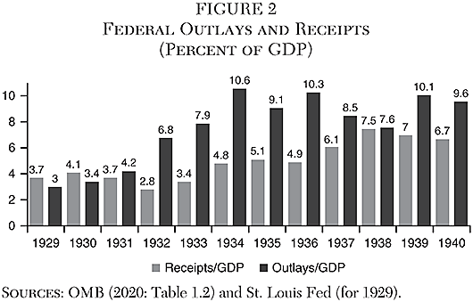
While tax rates were still low and exemptions high in 1929, the personal income tax brought in $1.18 billion, and it still raised $1 billion in 1930 when real GDP fell 8.5 percent (BEA 2020). When tax rates more than doubled in 1932 and exemptions were cut by $1,000, personal tax revenues dropped 46 percent—from $532 million in 1931 to $285 million in 1932 (BEA 2020). Despite a huge array of new and higher excise taxes—nearly tripling excise tax revenues in two years from $489 million in 1931 to $633 million in 1932 and $1,220 million in 1933 (BEA 2020: Table 3.2)—overall federal receipts nonetheless fell even faster than GDP—from 3.7 percent of GDP in 1931 to 2.8 percent in 1932 and 3.4 percent in 1933, as shown in Figure 2.

Higher personal income tax rates remained a symbolic political sideshow in terms of revenue in the Roosevelt years—raising just 1 percent of GDP from 1934 to 1940. Even in 1941, when the class tax began to be transformed into a mass tax with higher tax rates at lower incomes and reduced exemptions, individual income taxes still raised only 1.1 percent of GDP. But regressive excise and payroll taxes in 1941 amounted to 4 percent GNP (OMB 2020: Table 2.3).

Goolsbee (1999) investigates only the impact of higher noncorporate income tax rates on higher incomes in 1932 and 1936. He ­compares changes in incomes among three high‐​income groups over four‐​year spans that neither begin nor end during a year in which tax rates were changed. Like Romer and Romer’s long‐​term averages, this too leaves it unclear about what happened when tax changes took effect.

To estimate the effect of higher tax rates in 1932, for example, Goolsbee compares changes in the mean income of three groups of high‐​income taxpayers in 1931 with a Pareto‐​adjusted estimate of such incomes in 1935. There were apt to be changes in names attached to these incomes, however, since GDP fell sharply in 1930–31 and surged sharply in 1934–35. As Goolsbee (1999: 27) explains, “I purposely avoid using the base year as 1929 or 1930, because the output drops were much more dramatic in those years.” However, output did not drop in 1929. Moreover, there were also significant changes in 1934 tax rates on income and capital gains, so Goolsbee’s 1931–35 interval embraces two tax changes rather than one.

Goolsbee estimated ETI for the top two of the three groups as 0.24 and 0.31, due to negligible differences between those earning $25,000 to $50,000 and those earning $50,000 to $100,000. From the ETI estimates of 0.24 and 0.31, he deduces that the revenue‐​maximizing tax rate would be 83 percent if the tax system at that time had only one tax rate. That presumably means an 83 percent rate on all income above $25,000, rather than on all taxable income, but it clearly implies that Hoover’s 1932 tax increase could have maximized revenue if only marginal tax rates on those earning more than $25,000 had been 83 percent, which would have been almost double their actual (unweighted) average marginal rate of 47 percent.

Using such questionable ETI estimates to suggest the greatly increased 1932 marginal tax rates at high incomes were in any sense revenue maximizing, as both Goolsbee and Romer and Romer do, seems hard to reconcile with the deep, sustained drop in both income tax revenue and reported high incomes from 1932 to 1935.

Figure 2 shows that President Herbert Hoover increased federal outlays from 3 percent of GDP in 1929 to 8 percent in 1933.¹ As a share of GDP, Hoover increased domestic spending more than any president since 1902 except Nixon, according to Steuerle and Mermin (1997), and that was only partly because GDP fell in 1930–33.

President Hoover’s soaring spending and falling revenues raised the deficit from 0.5 percent of GDP in 1931 to 4 percent in 1932 and 4.5 percent in 1933. Since Keynesian convention defines “tax increases” by the amount of revenue raised, that approach cannot fathom how the counterproductive 1932 increases in tax rates could possibly have worsened the Depression, since revenues fell. By this standard, however, Hoover’s massive income tax rate increases could be reclassified as a massive tax cut (and “fiscal stimulus”) because income tax revenues fell.

In 1936, another increase in the highest tax rates was minor compared with an increase in dividend taxes at all incomes. Together, those tax hikes did appear to raise income tax revenues temporarily to $732 million in 1936 and briefly to $1.2–$1.3 billion in the 1937–38 recession. Several unique reasons for the procyclical tax increase in 1937–38 will be discussed later. After the 1937–38 recession, however, personal income tax receipts dropped back to $855 million by 1939 and barely reached $1.0 billion in 1940—slightly less than in 1930 and $154 million less than in 1929 (BEA 2020).

As a share of GDP, individual income taxes amounted to 1.1 percent of GDP in both 1929 and 1930, when tax rates were 1.1 percent to 25 percent, but then fell to an average of 0.7 percent of GDP from 1932 to 1935, when tax rates were 4 percent to 63 percent. Individual income tax receipts were still no more than 1.0 percent of GDP by 1939–40 when tax rates were 4 percent to 79 percent and personal exemptions had been slashed twice in 1932 and 1936 (BEA 2020).

To summarize: all the repeated increases in tax rates and reductions of exemptions enacted by presidents Hoover and Roosevelt in 1932–36 did not even manage to keep individual income tax collections as high in 1939–40 (in dollars or as a percent of GDP) as they had been in 1929–30. The experience of 1930 to 1940 decisively repudiated any pretense that doubling or tripling marginal tax rates on a much broader base proved to be a revenue‐​maximizing plan.

The most effective and sustained changes in personal taxes after 1931 were not the symbolic attempts to “soak the rich,” but rather the changes deliberately designed to convert the income tax from a class tax to a mass tax. The exemption for married couples was reduced from $3,500 to $2,500 in 1932, $2,000 in 1940, and $1,500 in 1941. Making more low incomes taxable quadrupled the number of tax returns from 3.7 million in 1930 to 14.7 million in 1940 (Piketty and Saez 2020: Table A0). The lowest tax rate was also raised from 1.1 percent to 4 percent in 1932, 4.4 percent in 1940, and 10 percent in 1941 (Tax Policy Center 2019a).

The percentage of adult households filing income tax returns rose from 6.4 percent in 1931 to 11.2 percent in 1938 and then jumped to 25.7 percent in 1940 and 45.8 percent in 1941 (Piketty and Saez 2020: Table A0). The income tax rate at an income of $10,000 rose from 11 percent to 14 percent in 1940, and at an income of $20,000, it rose from 19 percent to 28 percent. In other words, a rising share of middle‐​class income became taxable at higher tax rates after 1932, 1936, and 1940. But those with incomes above $50,000 could not or would not pay as much as they had in the 1920s, so the net result was no sustained increase at all in revenues from the individual income tax from 1929–30 to 1939–40.

Those earning less than $50,000 also faced higher tax rates after 1932, but their tax rates were increased only on dividends in 1936 (and another reduction in personal exemptions). Yet any resulting increase in revenues from middle‐​income taxpayers did not come close to offsetting the loss of income tax revenue from those earning more than $50,000, with the brief exception of higher taxes due from middle‐​income taxpayers in April 1937 on 1936 income from veterans’ bonuses and from dividends shifted from the (increased) corporate tax by the 1936 undistributed profits tax.

Figure 2 shows that federal receipts from all sources fell from 4 percent of GDP in 1931 to 3.2 percent in 1932, despite much higher excise taxes. By relying on ex ante estimates, however, Romer and Romer (2014: 245) depict revenues increasing $1,121 million in 1932 by more than 1.9 percent of GDP. If revenue had actually risen by 1.9 percent of GDP, as the Romer and Romer table suggests, then 1932 revenues would have been 5.9 percent of GDP rather than the actual ex post figure of 3.2 percent. In any case, the optimistic revenue estimate is almost irrelevant to Romer and Romer’s discussion on personal income tax changes in 1932, because only 16 percent ($178 million) of the Treasury’s additional revenue was estimated to come from higher individual tax rates and lower personal exemptions in 1932 (Thorndike 2003). Most was to come from higher excise taxes, which did rise by $731 million from 1931 to 1933.

If the ETI at high incomes had been nearly as low after 1932, as Goolsbee and Romer and Romer suggest, the much higher income tax rates at all incomes (and much smaller exemptions) would surely have raised much more individual income tax revenue from all income levels by 1940 than it had in 1929 ($1.2 billion). In fact, the individual income tax in 1940 raised no more revenue than much lower tax rates and larger exemptions raised during the 1930 slump.

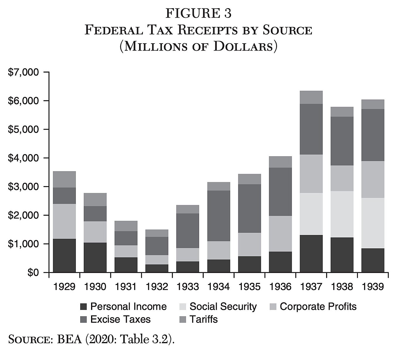
Total federal revenues from all sources did finally rise as a percentage of weakened GDP in the 1937–38 recession, as shown in Figure 2. Yet Figure 3 shows the increases in federal revenues after 1936 were mainly from increased excise taxes and new Social Security payroll taxes. Personal income tax receipts also rose in 1937 because taxes on 1936 income were due when tax returns were filed that April. But, as I will show, the 1936 spurt in taxable incomes was largely due to a $2 billion payout of taxable benefits to veterans in lower tax brackets and to a one‐​time payout of dividends made newly taxable at all incomes—rather than to higher marginal tax rates on high incomes.

Individual tax rates on dividends and high income were increased in the middle of FY 1936, which began June 1, 1935. Federal receipts only increased from 0.7 percent of GDP in FY 1935 to 0.8 percent in 1936, then 1.0 percent in 1937 and 1.4 percent in 1938, before falling back to 0.9 percent in 1940 (OMB 2020: Table 2.3). The increase in 1938 is somewhat illusory, the result of dividing small gains in revenue by big declines in GDP, because FY 1938 ended June 30, 1938, with four quarters of deep declines in real GDP. Revenue from high‐​income taxpayers in 1938 was boosted by a much lower 15 percent tax rate on capital gains that year, which encouraged realizations of accumulated capital gains, rather than to higher tax rates on other income. In fact, Figure 1 shows high incomes reported on tax returns falling sharply in 1937 and 1938, ending up lower than in 1935.

What happened when tax rates changed three times from 1934 to 1938 (in 1934, 1936 and 1938) is so complicated that Goolsbee and Romer and Romer do not agree. As Romer and Romer (2014: 266) write, Goolsbee’s results are “quite different” from theirs; he “finds an [elasticity] estimate that is large and negative while we obtain one that is large and positive.”

Goolsbee uses a relatively rapid increase in high incomes between 1934 and 1938 to approximate their response to higher tax rates in 1936. The trouble is there were three major changes in federal taxes from 1934 to 1938, not just one.

Romer and Romer cannot resolve their 1934–38 differences with Goolsbee, because their elasticities “cannot be estimated with any useful degree of precision (particularly in 1934 and 1938)”—ranging from zero to 3.0 for 1934, zero in 1936, and about minus 2.8 to plus 2.2 in 1938 (Romer and Romer 2014: 266–67). Their problem with 1934 and 1938 is that (unlike Goolsbee) they exclude capital gains from income and thus exclude unprecedented changes in capital gains tax rates in both 1934 and 1938. Goolsbee counts capital gains as income but misinterprets a one‐​time 1938 surge in high‐​income gains as a negative taxpayer response to 1936 tax rates on ordinary income rather than a positive response to a new 15 percent tax rate on capital gains.

Until 1933, the capital gains tax was 12.5 percent on assets held more than 2 years. In 1934–37, capital gains on asset sales were ­subject to a schedule of steep tax rates, depending on how long an asset was held (Reynolds 2015). The tax rate was reduced from 80 percent to 60 percent of a taxpayer’s marginal rate for assets held for 2 to 5 years, then 40 percent after 5 years, and 30 percent after 10. At an income of $100,000, the marginal tax rate was 56 percent in 1934 and 62 percent in 1936. The capital gains tax on an asset held 2 to 5 years was therefore at least 33.6 percent in 1934 and 37.2 percent in 1936.

Taxpayer decisions to realize capital gains by selling appreciated assets are famously hypersensitive to the largely voluntary tax paid by those who make that decision. In 1933, taxpayers earning more than $100,000 realized $97.1 million of long‐​term capital gains. Statistics of Income (SOI) could not cope with multiple taxes on capital gains from 1934 to 1937, so they lumped short‐​term and long‐​term gains together. Total capital gains at incomes above $100,000 promptly collapsed to $22.9 million in 1934. After 1936, with even higher capital gains tax rates on high incomes, total short and long‐​term capital gains fell to $3.3 million in 1937.

Shortly before June 1938, Congress slashed the capital gains tax on assets sold after two years from to 15 percent. In that year, taxpayers with income above $100,000 realized $134.8 million in capital gains, up from $3.3 million the year before. In the year Goolsbee chose to illustrate no response at all of high‐​income taxpayers to changing marginal tax rates, high‐​income taxpayers chose to respond quite forcefully to a lower marginal tax rate on capital gains.

The elasticity of capital gains realizations is famously high (about 1.0), because if you rarely sell assets you rarely pay the tax. The collapse of asset sales when the capital gains tax went up in 1934 easily dwarfed later effects of a modest 1936 rise in the slice of ordinary income that exceeded $50,000. Total IRS income above $100,000 (including capital gains) rose by $111 million from 1934 to 1938—from $419.8 million to $530.8 million (SOI Stats Archive). However, capital gains alone in that top‐​income group rose slightly more than total income did—by $111.9 million—from $22.9 million in 1934 to $134.8 million in 1938.

A relatively larger income gain for those reporting incomes of $100,000 led Goolsbee to claim the ETI was negative in response to higher top tax rates in 1936. That is why he claimed a flat tax of 100 percent in 1936 could have been revenue maximizing. Yet, all of the 1934–38 increase in incomes above $100,000 happened because the tax on two‐​year capital gains was reduced from 38–47 percent in 1937 to 15 percent in 1938—not because of a minor tax rate increase on other sources of income two years earlier.

Despite the 1938 surge of capital gains at incomes above $100,000, amounts reported by many more returns with taxable income above $50,000 in Figure 1 only totaled $1.11 billion in 1935, $1.89 billion in 1936, $1.69 billion in 1937, and below $1 billion in 1938. Taxable high incomes were just not large enough to explain why receipts from the individual income rose to 0.8 percent of GDP in 1936, 1.0 percent in 1937, and 1.4 percent in 1938. Besides, the total of high incomes on tax returns moved in the wrong direction from the ratio of receipts to GDP—falling from 1936 to 1938 rather than rising.

Viewed as a percentage of GDP, federal taxes collected from individual incomes at all incomes appear to rise during the recession of 1937 and 1938 when incomes were falling half the time. This was not because raising the marginal tax rate from 34 percent to 35 percent on $50,000 incomes in 1936 brought in a ton of revenue. It was because taxable income suddenly increased at all incomes in 1936, particularly middle incomes. And income earned in 1936 was taxed when returns were filed in April 1937, while most income earned in 1937 was likewise taxed in 1938.

Very little of the added revenue collected in 1937–38 came from those earning more than $50,000, whose marginal tax rates were (slightly) increased. The high‐​income share of income tax receipts fell in 1937 when those receipts peaked.

Aside from some residual monetary stimulus—with nominal GDP rising by 14.3 percent largely because of the 1934 devaluation (Eggertsson 2008; Sumner 2015: chap. 7)—most of the ephemeral spurt in taxable income at all incomes in 1936–37 was unique and uncomplicated. It happened because of (1) an enormous one‐​time payment of veterans’ bonuses; (2) shrinking tax exemptions and bracket creep; (3) income shifting from corporate to individual tax forms due to a new corporate tax on earnings not distributed as dividends; and (4) higher tax rates due for the first time from all taxpayers in 1937 on artificially large dividends received in December 1936 from income shifting.

On January 24, 1936, Congress passed, over the president’s veto, a World War I veterans’ bonus, which paid $1.76 billion in $50 bonds to 3.2 million veterans—80 percent of which was redeemed in 1936, particularly from June 15 to July 31(Hausman 2016: 1105). Veterans’ bonuses affected nearly 8 percent of all households and amounted to 2 percent of GDP and at least 30 percent of average income (which was about $1,500) for those aged 35 to 44 (Tesler 2003). The average bonus was $581, enough to buy a new car or make a down payment on a house, so sales of consumer durables and homes boomed.

Because the personal exemption was reduced to $1,000 for singles and $2,500 for couples in 1936, many veterans’ bonuses were taxable income for people with incomes (even including the bonus) that were modest. There were 33 tax brackets in 1936, so 3.6 percent inflation that year caused some “bracket creep” by pushing even $2,000 increases in nominal income into a higher tax bracket.

The Revenue Act of June 22, 1936, also introduced a crucially important graduated surtax of 12–27 percent on undistributed corporate profits. It caused rapid, large “income shifting” from the corporate tax to individual tax by encouraging corporations to increase dividend payouts to escape the tax in 1936–37 (Haas 1937). Income shifting, in turn, contributed to low elasticity estimates for 1936 from Romer and Romer and Goolsbee, because it briefly boosted the share of corporate income reported on high‐​income shareholder individual tax returns (rather than on corporate returns). Part of what would otherwise have been counted as retained corporate income was briefly reported and taxed as increased dividends at the individual level in 1936 when dividend tax rates at all income levels were substantially increased. Piketty and Saez (2020: Table A7) find that as a percentage of reported taxable income of the top 10 percent (virtually all taxpayers), dividends rose from 12.5 percent in 1934–35 to 15.7 percent in 1937–38, then fell to 11.5 percent in 1938 when tax rates on retained earnings and capital gains fell.

Before 1936, most taxpayers facing low tax rates of 4–8 percent were exempt from any tax on dividends, and others subtracted the 8 percent rate from their rates. The top rate of 63 percent was 55 percent for dividends. The surge of dividends, distributed to individuals in 1936 (to avoid the new corporate tax on retained earnings), were newly subjected to combined basic and surtax rates of up to 79 percent. What is more important for explaining the 1936–37 surge in ­taxable income, dividends became widely taxable for the first time even for those in the lowest tax brackets.

Federal revenue from all sources were only 4.6 percent of GDP in 1936 (similar to 1930), but then rose to 5.8 percent in 1937 and 7.7 percent in 1938 (Figure 2). Taxes on incomes earned in 1936 were not due until April 1937. But even in 1937, the peak individual income tax of $1.3 billion in 1937 was still only 26 percent of federal revenue—smaller than the new Social Security tax ($1.47 billion) or excise taxes ($1.77 billion).

An ephemeral 12.8 percent spurt in real GDP in 1936 led by consumer spending (of bonus checks) was promptly followed by deep recession from May 1937 to June 1938, cutting GDP by 10 percent and industrial production by 32 percent, with unemployment rising to 20 percent.

At the time of what critics dubbed the “Roosevelt Recession” economists like Joseph Schumpeter and industrialists like Lammot du Pont “severely criticized … the undistributed profits taxes and capital gains taxes” (Roose 1954: 209–16). The Democratic Congress feared voter backlash that fall (when they did lose 72 seats in the House and 7 in the Senate), so on May 28, 1938, Congress greatly reduced or repealed these unpopular taxes and the economy rebounded.

The undistributed profits tax went into force in June 1936, but its effects on corporate profits and liquidity were not apparent, Schumpeter noted, until the first quarter of 1937. Corporations avoided paying the tax by a huge dividend payout in December 1936, which briefly added to personal income in 1936 before adding to taxes due on April 1937. But retaining no earnings left firms precariously short of liquidity and dependent on external funds for investment, which was difficult or impossible for small firms and costly for large ones.

High taxes on capital gains discouraged risky ventures, du Pont argued and Roose agreed. But because he mistakenly thought the capital gains tax rates in 1936–37 were the same as in 1934 (they rose at incomes above $50,000), Roose concludes that “only the social security and undistributed profits taxes appears to have had a direct influence on the timing and occurrence of the recession” (Roose 1954: 215).

The Revenue Act of May 28, 1938, passed without the president’s signature. That law slashed tax on undistributed profits to 2.5 percent in 1938 and abolished it in 1939. The top tax on capital gains was cut to only 15 percent on assets held two years. The higher discounted present value of future after‐​tax earnings was quickly capitalized as the Dow Jones stock index rose from 107.9 the day before the tax cut to 130.5 a month later and 154.8 by the end of the year (Johnston and Williamson 2019).

With confidence and wealth on the rise, the recession ended in June—a few days after the 1938 tax cuts. Yet Romer and Romer (2014), among others, argue that massive increases in numerous income and excise taxes in 1932–36 had no ill effects on the U.S. economy.

In a renowned 2010 paper about 1945–2007, Romer and Romer (2010: 763, 781) concluded that “tax increases are highly contractionary,” and “have a very large, sustained, and highly significant negative impact on output.” They also found the prolonged “persistence of the effects [on investment] is suggestive of supply effects” on incentives (ibid.: 799).

By contrast, the 2014 Romer and Romer estimates of a low ETI in prewar years, and their related high estimates of revenue‐​maximizing income tax rates, may appear to demonstrate that higher tax rates were not harmful to the weak and unstable economy of 1932–38. But that would be an unduly broad conclusion to base on such narrow evidence. The Romer and Romer ETI estimates deal exclusively with only one relatively small federal tax (the personal income tax accounted for only 15.3 percent of federal revenue in 1933) and on too small a number of taxpayers (about 25,000) to capture the impact of all the increased taxes on capital, labor, and sales enacted in 1932 and 1936.

Romer and Romer (2014: 278) nonetheless examine connections between increases in top marginal income tax rates and select measures of short‐​term business activity. They find “no evidence of an important effect of changes in marginal income tax rates on machinery investment and industrial construction.” Importantly, they assume no “effects on long‐​run economic performance” and, instead, focus on “immediate” or “temporary” effects on two minor indicators of business investment.

In 1932, real investment in business equipment fell 41.1 percent, structures by 38.8 percent, and housing by 43.5 percent (BEA 2020). Growth theory and real business cycle theory might suggest that collapse of fixed investment was at least aggravated by greatly increased 1932 corporate and personal tax rates on expected future returns from investment. Yet Romer and Romer (2014: 278) see “no evidence that the large swings in the after‐​tax share in the interwar era had a significant impact on investment in new machinery or commercial and industrial construction.” Indeed, they report that, “Machinery production … changed little immediately after the very large 1932 tax increase “(ibid.: 273). Also, “commercial and industrial construction contracts … changed little following the 1932 tax increase, and rose temporarily after the 1935 tax increase”—which actually took effect in 1936.

Rather than concentrating on how machinery production fell (after orders declined), a more forward‐​looking indicator of a tax shock would be manufacturers’ new orders for such durable goods, just as construction contracts are a leading indicator of actual construction (which does not usually stop until projects are completed). The forward‐​looking NBER index for manufacturers’ new orders for durable goods fell to 34 in 1932 from 60 in the previous year.² And regardless what may have happened temporarily to construction contracts, nonresidential construction spending was cut in half in 1932—from over $1 billion in 1931 to $502 million in 1932; it fell further to $406 million in 1934 (BLS 1953: 9).

Romer and Romer (2014: 275) trend‐​adjust some of their investment proxies “to help address the fact that there were enormous macroeconomic fluctuations in this era.” They make these cyclical adjustments by estimating “how investment behaves in the wake of changes in tax rates given the path of overall economic activity following the changes.” They claim such cyclical adjustment of investment data is “reasonable if the effects of the tax changes on the overall economy are small … in light of their small impact on aggregate demand.” That alleged “small impact on aggregate demand” implies that because Hoover’s 1932 tax increase did not raise revenue or reduce the deficit (the opposite in fact), it must have been a fiscal stimulus rather than contractionary within a vintage Keynesian narrative linking budget deficits to nominal GDP growth.

Even within that narrative, however, Figure 3 shows that increases in total federal tax revenues in the 1930s were dominated by payroll and excise taxes. These broad‐​based taxes on what people earn and spend cannot easily be dismissed as having had a “small impact on aggregate demand.” Cole and Ohanian (1999: 6) found “consumption fell about 25 percent below trend and remained near that level for the rest of the decade.” This should not be surprising at a time when federal excise taxes alone were at a peacetime record high and many states added or increased sales taxes.

When Romer and Romer (2014) judge the effect of changed income taxes (rather than excise and payroll taxes) by their “fairly small [and sometimes inverted] effects on revenues,” they refer to and depend upon estimated changes in revenues—“statements about the expected revenue effects of a tax change at the time it was scheduled to go into effect.” They inform readers that the 1932 tax law was estimated to raise revenues by 1.9 percent of GDP as though estimated revenue was meaningful, even though actual revenues fell by 0.8 percent of GDP that year.

Romer and Romer speak of “large swings in output” and “enormous macroeconomic fluctuations” in the 1930s as if two depressions in eight years were entirely due to Fed policy or bad luck and not at all to destructive tax, trade, or regulatory policy. “It is difficult to separate the effects of tax changes from the large cyclical movements in investment,” Romer and Romer (2014: 243) acknowledge. Yet to dismiss huge movements in investment as merely cyclical—or to obscure such movements with trend adjustments—tends to minimize possibly damaging effects of tax changes on business and household investment. Moreover, to focus solely on questionable indexes of short‐​term investment and construction also neglects many other disincentive effects of higher tax rates on productive activity. Akcigit and Stantcheva (2020: 6), for example, find “that both corporate and personal income taxes negatively affect the quantity and quality of innovation at the macro state level and the individual inventor and firm levels.”

In marked contrast to what Stein, Burns, and Brown once said about Herbert Hoover’s suicidal tax increases in 1932, Cole and Ohanian (1999: 12) recently wrote that “tax rates on both labor and capital changed very little in 1929–33, which implies that they were not important for the decline.” Yet marginal personal tax rates on both labor and capital (e.g., small business and partnership income, dividends, interest, rent, and capital gains) were greatly increased in 1932 on everyone who was not exempt and exemptions were reduced. Marginal excise tax rates were greatly increased in 1932 and 1936. The effective corporate tax rate was increased from 11 percent in 1929 to 13.75 percent in 1932, 17.6 percent in 1937, and 19 percent in 1938 (Seater 1982: 363).

The 1932 tax law involved raising the top tax rate from 25 percent to 63 percent, quadrupling the lowest rate from 1.1 percent to 4 percent, and increasing corporate and estate tax rates. It is important to realize that federal excise and state sales tax rates also affect marginal rates on factor incomes, and both rose in the 1930s. Hoover’s 1932 tax was mainly about broader and higher excise taxes on goods and services. Those increased excise taxes (as well as the infamous tariffs of 1930) ultimately fell on factor incomes. Taxes on the uses of income, like taxes on the sources of income, reduce after‐​tax rewards to people who supply the complementary factors of labor and capital.

To focus exclusively on marginal tax rates on only personal income and at only the federal level, clearly understates the increases in marginal tax rates on income and sales at the federal, state, and local levels. In an understatement, Romer and Romer (2012: 15–16) briefly mentioned in their background notes that “the majority of the [estimated] revenue effects were due to a vast increase in excise taxes. The most notable of these was an across‐​the‐​board tax of 2¼ percent on all manufactured articles.”

The revenue‐​maximizing top tax rate formula that Romer and Romer borrow from Diamond and Saez (2011: 168) was never intended to be a top rate for the federal income tax alone as they imply, but to include all taxes on income, payrolls, and sales at the federal, state, and local levels. Even for the narrow purpose of estimating revenue‐​maximizing tax rates, it is a serious omission for Romer and Romer and Goolsbee to ignore federal and state excise and sales taxes, as well as state income and sales taxes. In fact, to focus only on the economic impact of the federal tax on individual incomes in 1932–40 is to leave out 92.5 percent of all federal, state, and local tax receipts in those years (BEA 2020: Tables 3.4 and 3.5).

In 1932, federal income tax rates were roughly doubled at all income levels, with larger increases at the lowest and highest incomes. In 1934–36, there were additional increases in income taxes on capital gains and dividends, and marginal tax rates were again increased on net incomes of $50,000 or more. In 1929, the federal income tax on individuals accounted for 50.9 percent of all federal taxes and 14.1 percent of all federal, state, and local taxes. From 1932 to 1940, by contrast, the federal income tax accounted for an average of 25.8 percent of all federal taxes and only 7.5 percent of total federal, state, and local taxes (BEA 2020: Tables 3.4 and 3.5). If the objective of high marginal tax rates on personal income from labor and capital was to maximize revenue, regardless of any adverse impact on growth of the economy (and therefore growth of taxable income), the Hoover and Roosevelt plans to fix the Depression with higher taxes in 1932–36 were a total failure.

To point out that high and rising federal income tax rates in 1932–36 reduced revenue from $1,179 million in 1929 to $855 million in 1939, certainly does not imply that steep marginal tax rates were small in terms of distortions, disincentives, or tax avoidance. On the contrary, the decade‐​long inverse relationship between tax rates and revenue suggests high tax rates were extremely inefficient, causing large deadweight costs with no lasting revenue gain. The greatly increased tax rates on realized capital gains from 1934 to mid‐​1938 are a good example. By discouraging asset trading, high tax rates on realized gains (47 percent after two years) reduced realizations and tax receipts. Falling tax receipts, in turn, makes those higher tax rates look unimportant in terms of static bookkeeping and Keynesian macroeconomics. Yet falling revenue from higher tax rates illustrates the high cost of punitive marginal tax rates with no offsetting benefits.

Despite large increases in many such distortive federal and state marginal tax rates on what people earn and on how they spend those earnings, Mulligan (2002) nonetheless relies only the federal tax on individual labor income to agree with Cole and Ohanian that new taxes on labor and capital were trivial and insignificant in 1932–33 (and Mulligan includes 1936–38). He remarks that

Cole and Ohanian (1999) suggest that … taxes on factor incomes might help explain some of the Depression economy.… Of course, taxes on labor income create such a wedge, but Barro and Sahasakul’s study suggests that federal taxes on payroll and individual income were trivial, and unchanging.… [The] vast majority of the population did not file ­individual income tax returns during the 1930s, so that any IRS‐​induced tax wedge affected very few people (not to mention small effects for the few affected) [Mulligan 2002: 27].

Mulligan emphasizes only the labor tax wedge (without mentioning the 1937 payroll tax) while neglecting marginal tax rates on capital incomes: higher corporate tax rates, surtaxes on undistributed profits, higher individual tax rates on partnerships and small enterprises, higher tax rates on capital gains in 1934–37, on dividends in 1936, and raising the top tax on estates from 20 percent in 1931 to 70 percent 1936.

Wright (1969: 300) estimates the average U.S. marginal tax rate on dividends rose from 11.1 percent in 1928 to 27.1 percent in 1932 and 29.9 percent in 1936, and the marginal tax on interest income rose from 9.2 percent in 1928 to 14.4 percent in 1932 and 17.6 percent in 1936. Federal taxes on gifts and estates rose from $35 million in 1932 to $379 million in 1936—nearly half as large as the $732 million collected that year from individual income taxes (Joulfaian 2007: Table 6).

The only reason both Mulligan and Cole and Ohanian imagine nothing significant happened to tax policy in the 1930s is that both rely entirely on inappropriate or irrelevant estimates of an income‐​weighted “average” of marginal tax rates from the federal individual income tax alone.

To explain why they suppose “tax rates on both labor and capital changed very little 1929–33,” Cole and Ohanian cite a 1981 study by Joines, which shows average marginal rates on labor little changed until 1937 when the Social Security tax was added. Mulligan (2002) cites similar 1983 estimates from Barro and Sahasakul (1983). Yet, Barro and Sahasakul were highly critical of the income tax rate increases of 1932 and 1936, which they explained in detail. They wryly concluded: “Apparently the tax increases between 1932 and 1936 reflect the Hoover‐​Roosevelt program for fighting the Depression!” (Barro and Sahasakul 1983: 21).

Barro and Sahasakul (ibid.: 1) “argue that the explicit rate from the schedule is the right concept for many purposes.” And those rates, they explicitly explained, were greatly increased between 1932 and 1936. Yet the same authors’ income‐​weighted “average marginal tax rate” fell from 4.1 percent in 1928 to 2.9 percent in 1932 and 3.1 percent in 1933. That is why Mulligan (2002: 27) concludes, “Barro and Sahasakul’s study suggests that federal taxes on payroll and individual income were trivial, and unchanging.” On the contrary, Barro and Sahasakul (1983: 1) derided higher income tax rates in 1932 and 1936 and apologized for not including payroll taxes (until later). They also apologized for excluding excise taxes. “A full measure of marginal tax rates,” they wrote, “would incorporate other levies, some of which are based on property or expenditures” (ibid: 2). Increased federal expenditure (excise) taxes on dozens of good and services directly affected millions more people than the individual income tax, and excise taxes brought in over twice as much revenue (an average of $1,536 million per year from 1932 to 1939 compared with $728 million for the income tax).

The seemingly paradoxical decline from 1928 to 1932 in the Barro and Sahasakul “average marginal tax rate” does not show that marginal tax rates fell in 1932 or were either trivial or unchanging. What it does show is that the 1928–29 income‐​weighted average was heavily weighted toward a rising number of high incomes above $50,000 taxed at rates of 18–25 percent, while the 1932–35 average was instead heavily weighted toward many more low incomes taxed at 4–10 percent (up from 1.5–5 percent in 1931).

As Seater (1982: 354) explained, an “income‐​weighted average marginal rate” is computed by “using for weights the fraction of income that fell within each income class.” Because very little income still fell into the high‐​income tax brackets after 1932, the weight of high‐​tax brackets within the average was diluted. This is an entirely different concept of “average marginal rate” than I used in Figure 1, which is an unweighted average of statutory rates.

Income‐​weighted averages of marginal tax rates in this period are a roundabout way of describing the same phenomenon as Figure 1—namely, that many high incomes dropped out of those averages after 1932. Reported net incomes above $50,000 collapsed from $6.3 billion in 1928 to $800 million in 1932 and never again even hit $2 billion before WWII. As billions of dollars of high taxable incomes vanished when faced with the high 1932–35 marginal tax rates, all the income‐​weighted “average marginal tax rates” became dominated by much larger weights then attached to numerous taxpayers with relatively inelastic lower incomes.

Mulligan focuses on the fact that few people paid federal income tax after 1932—especially fewer high‐​income people—than before. Yet it is also true that relatively few people start new businesses, employ many people, or supply capital to those who do. As McGrattan (2012: 2) notes, “Although few households paid income taxes, those who did earned almost all of the income distributed by corporations and unincorporated businesses. If the increases in rates were not completely unexpected [Hoover announced them in December 1931], these households would have foreseen large declines in future gross returns on investments … even before 1932 when major changes were enacted.”

When it comes to blaming the Depression’s severity and length partly on bad tax policy, McGrattan and others remain somewhat closer to the early postwar consensus of Stein, Burns, and Brown. McGrattan assigns considerable blame for the stubborn severity of the post‐​1932 depression in general, and 1937–38 recession in particular, on high marginal corporate and individual tax rates on capital. That includes new taxes on retained earnings and higher taxes on dividends in 1936, plus high tax rates on most realized capital gains from 1934 until early 1938.

Calomiris and Hubbard (1995) also find the 1936–37 surtax on undistributed corporate profits was particularly harmful to the working capital and plant and equipment outlays of smaller, rapidly growing firms. Large corporations could avoid the tax by paying more dividends (reported as taxable income on individual income tax returns), but this was not a viable option for smaller growth companies with limited access to external funds and therefore dependent on retained earnings to reinvest for expansion.

Christina Romer (2009) blames the 1937–38 economic collapse partly on the new payroll tax for Social Security, which raised even more revenue that year ($1,473 million) than the briefly engorged personal income tax ($1,305 million), although not as much as newly increased excise taxes ($1,771 million). Cole and Ohanian (1999: 12) estimate that increases in the marginal tax on labor between 1929 and 1939 (notably the payroll tax) reduced the steady‐​state labor supply by 4 percent.

Mulligan (2002) does acknowledge that excise taxes fall on the income received from supplying labor and capital and could ­therefore raise marginal tax rates on factor income.³ However, he mistakenly compares today’s minor excise taxes (0.4 percent of GDP) with those of 1932–40 (2.1 percent of GDP). He writes, “The federal government did not have a general sales tax, although it does have (and has had) excise taxes on goods such as cigarettes, gasoline, and imports. However, the revenues from these taxes are [today] too few, and not changing enough over time, to drive much a of wedge” (ibid.: 25). On the contrary, excise taxes that were added and increased in 1932 and 1936 were neither few in number, small in size, nor modestly changed (see Figure 3).

In 1932, the secretary of the Treasury reported that the Revenue Act of 1932 “effected one of the largest increases in taxes ever imposed by the federal government.” The report boasted of “manufacturers’ excise taxes on numerous articles” and “other miscellaneous taxes, including new and increased stamp taxes, increased taxes on admissions, and new taxes on telephone, telegraph, cable, and radio messages, checks, leases of safe deposit boxes, transportation of oil by pipe line, and the use of a boat” (U.S. Treasury 1932: 21).

Excise tax receipts in 1933 were $1.58 billion—up from $532 million in 1931 and more than four times the $390 million collected from high personal income taxes. From 1932 to 1939, individual income taxes averaged less than 1 percent of GDP, but excise taxes were 2.1 percent of GDP (OMB 2020: Table 2.3).

In a survey about the theory and evidence of economic growth, Robert Barro and Paul Romer (1990: 3–4) concluded that “all economic improvement can be traced to actions taken by people who respond to economic incentives .… If government taxes or distortions discourage the activity that generates growth, growth will be slower.”

News about abrupt changes in government taxes (or regulatory distortions) may create a policy shock forcing the people to respond to new incentives. Using postwar data, for example, McGrattan (1994: 25) finds “tax rate shocks have a significant effect on the variance of most of the variables in the model” including consumption, output, hours worked, capital stock, and investment. In simulations by Sirbu (2016: 24), changing “news about [future] capital income tax rates … generate not only qualitatively but also quantitatively realistic aggregate fluctuations.”

Few economic historians who have written about causes of the Great Depression have assigned much importance to tax changes, and many entire books on the subject do not even mention tax policy. In the late 1930s and early postwar decades, however, ­economists commonly agreed that large increases in personal, corporate, and excise tax rates in 1932 and 1936 contributed to the Depression. This article reviews more recent and very different studies that assert or imply that tax rate shocks in the 1920s and 1930s had no discernible impact on activity that generates growth.

Romer and Romer (2014) and Goolsbee (1999) investigate whether reductions in the highest marginal tax rates during the 1920s encouraged high‐​income taxpayers to earn and report more income and, conversely, whether higher top tax rates in 1932 and 1934–36 encouraged affluent taxpayers to report less income. Figure 1, by contrast, shows high incomes always moved inversely with marginal tax rates (except in 1936–38) suggesting elasticity of taxable income (ETI) was high.

Romer and Romer conclude otherwise, as does Goolsbee for 1930s. They claim ETI was so low in 1932–38 that top tax rates of 73–84 percent would have been revenue maximizing. Yet raising the top tax rate from 25 percent in 1925–31 to 63–79 percent in later years produced individual income tax revenues no higher in 1940 than they had been in 1930.

Goolsbee and I agree that the ETI was high when such tax rates were greatly reduced in 1923–26. But where I find substantial qualitative response after tax rates rose sharply in 1932, and Romer and Romer find a middling ETI of 0.42, Goolsbee finds a weak taxpayer response (0.27) from 1931 to 1935, which is his proxy for what happened in 1932. He also finds the highest incomes rose 1934 to 1938, which he interprets as zero response to higher tax rates in 1936. But I show that was because capital gains realizations collapsed in 1934 when the capital gains tax was greatly increased then surged in 1938 as that tax was cut to 15 percent.

Romer and Romer’s low ETI estimates for tax rate reductions in 1924 and 1926 assume (doubtfully) that taxpayers could not anticipate those preannounced rate cuts would be retroactive. Elasticities for tax changes in 1934–38, they say, “cannot be estimated with any useful degree of precision” (Romer and Romer 2014: 266).

To buttress their ambiguous ETI estimates for 1932–38, Romer and Romer offer a benign interpretation of the 1932 tax law’s economic impact, finding few immediate effects on select measures of business activity and assuming no effect on aggregate demand. That exercise is inherently incomplete because it (1) includes only about 25,000 taxpayers and (2) excludes major changes in excise taxes and in tax rates on dividends in 1936, capital gains in 1934–37, and undistributed corporate profits in 1936–37. I argue that what happened to those widely ignored taxes largely explains the brief anomaly of high incomes and top tax rates moving up together in 1936–38 (e.g., a temporary spike in dividend payouts in 1936 and surge in capital gains in 1938) as well as the simultaneous recession of late 1937 and early 1938 (see McGrattan 1994).

Cole and Ohanian (1999) and Mulligan (2002) do not merely claim higher tax rates were harmless (as Romer and Romer do) but claim there were no significant changes in marginal tax rates on labor or capital in 1932 or 1936. That puzzling claim depends entirely on inapt estimates of income‐​weighted “average marginal tax rates,” which fell when all statutory tax rates rose. That is because these are averages of tax rates weighted by the number of tax returns in low, middle‑, or high‐​income groups. After top tax rates rose from 25 percent to 63–79 percent in 1932 and 1936, the so‐​called average marginal tax rates assigned much less weight to the shrinking numbers of taxpayers in higher tax brackets in 1932–39 than they had before. In 1928, 43,184 taxpayers with gross incomes above $50,000 accounted for 11 percent of all tax returns. In 1935, high‐​bracket taxpayers accounted for only 10,680 (0.02 percent) of 4.6 million returns (SOI). Far from proving weak response to high tax rates, vanishing high incomes illustrates the opposite (i.e., high ETI).

To focus on the federal tax on individual incomes alone, as all these studies do, misses a much bigger picture. Federal taxes were a small fraction of total government revenues (29.3 percent from 1932 to 1940) and the individual income tax was a small and shrinking fraction of that small federal share. The 1932 and 1936 revival of wartime excise taxes on a huge array of goods and services was enormously damaging to aggregate demand (sales taxes reduce sales) and factor supply (sales taxes are paid from after‐​tax returns to labor and capital). By 1940, the individual income tax accounted for only 13.6 percent of federal revenue, the corporate tax for 18.3 percent, Social Security tax for 27.3 percent, and excise taxes for 30.2 percent (OMB 2020: Table 2.2).

After presidents Hoover and Roosevelt embraced what Herb Stein dubbed “the desperate folly of raising taxes in a Depression,” ­individual income taxes amounted to “1.4 percent of personal income in 1929 and only 1.2 percent in 1939” (Stein 1988: 58). It turned out that, contrary to revenue‐​maximization simulations of a 74–83 percent top tax rate by Goolsbee or Romer and Romer, a top tax rate of 25 percent on personal income (and 12.5–15 percent on capital gains) proved to be the long‐​run revenue‐​maximizing top tax rate of 1918–40.

A previous critical review of estimates of the ETI at high incomes in the postwar years found those estimates far too low and found the authors’ arguments about tax rates being unrelated to economic growth factually flawed (Reynolds 2019). This review of prewar ETI estimates finds them equally understated and also too constricted—dealing with only a tiny fraction of many federal and state taxes on labor and capital. Artificially low ETI estimates for the 1920s and 1930 as well as an income‐​weighted average of marginal tax rates have both been used to claim that exceptionally large and increasingly regressive tax increases from 1932 to 1937 had nothing to do with two deep recessions in those years. That is too strong a conclusion to be supported by such weak evidence.

Akcigit, U., and Stantcheva, S. (2020) “Taxation and Innovation: What Do We Know?” Becker Friedman Institute, Working Paper No. 2020–70, University of Chicago (May 6).

Barro, R. J., and Romer, P. M. (1990) “Economic Growth.” NBER Reporter (Fall).

Barro, R. J., and Sahasakul, C. (1983) “Measuring the Average Marginal Tax Rate from the Income Tax.” NBER Working Paper No. 1060 (January).

BEA, Bureau of Economic Analysis (2020) “GDP and Personal Income” and “Federal Government Current Receipts and Expenditures” Tables 3.2–3.5 (May 28). Interactive data available at https://​apps​.bea​.gov/​i​t​a​b​l​e​/​i​n​d​e​x.cfm.

BLS, Bureau of Labor Statistics (1953) “Construction during Five Decades, Historical Statistics, 1907–52.” Bulletin No. 1146 (December 15).

Brown, E. C. (1956) “Fiscal Policy in the ‘Thirties: A Reappraisal.” American Economic Review 46 (5): 857–79.

Burns, A. (1958) Prosperity without Inflation. Buffalo, N.Y.: Economica Books.

Calomiris, C. W., and Hubbard, R. G. (1995) “Internal Finance and Investment: Evidence from the Undistributed Profits Tax of 1936–1937.” Journal of Business (October): 443–82.

Cole, H. L., and Ohanian, L. E. (1999) “The Great Depression in the United States from a Neoclassical Perspective.” Federal Reserve Bank of Minneapolis Quarterly Review 23 (1): 2–24.

de Rugy, V. (2003) “Tax Rates and Tax Revenue: The Mellon Income Tax Cuts of the 1920s.” Tax & Budget Bulletin 13 (February). Washington: Cato Institute.

Diamond, P., and Saez, E. (2011) “The Case for a Progressive Tax: From Basic Research to Policy Recommendations.” Journal of Economic Perspectives 25 (4): 165–90.

Eggertsson, G. B. (2008) “Great Expectations and the End of the Depression.” American Economic Review 98 (4): 1476–516.

Frenze, C. (1982) “The Mellon and Kennedy Tax Cuts: A Review and Analysis.” Joint Economic Committee Staff Study (June 18).

Goolsbee, A. (1999) “Evidence on the High‐​Income Laffer Curve from Six Decades of Tax Reform.” Brookings Panel on Economic Activity (September 26). Available at https://​fac​ul​ty​.chicago​b​ooth​.edu/​a​u​s​t​a​n​.​g​o​o​l​s​b​e​e​/​r​e​s​e​a​r​c​h​/​l​a​f.pdf.

Gwartney, J. D. (2002) “Supply Side Economics.” In D. R. Henderson (ed.), The Concise Encyclopedia of Economics. Indianapolis: Liberty Fund.

Haas, G. (1937) “Rationale of the Undistributed Profits Tax.” U.S. Treasury Department Staff Memo (March 17). Available at www.taxhistory.org/Civilization/Documents/UPT/HST8668/hst8668‑1.html.

Hausman J. H. (2016) “Fiscal Policy and Economic Recovery: The Case of the 1936 Veterans’ Bonus.” American Economic Review 106 (4): 1100–43.

Johnston, L., and Williamson, S. H. (2019) “What Was the U.S. GDP Then?” Available at www​.mea​sur​ing​worth​.org/​usgdp.

Joulfaian, D. (2007) “The Federal Gift Tax: History, Law, and Economics.” U.S. Department of the Treasury, OTA Paper 100 (November).

McGrattan, E. R. (1994) “The Macroeconomic Effects of Distortionary Taxation.” Journal of Monetary Economics 33 (3): 573–601.

________ (2012) “Capital Taxation during the U.S. Great Depression.” Quarterly Journal of Economics 127 (3): 1515–50.

Mulligan, C. B. (2002) “A Dual Method of Empirically Evaluating Dynamic Competitive Equilibrium Models with Distortionary Taxes, Including Applications to the Great Depression and World War II.” NBER Working Paper No. 8775 (February).

OMB, Office of Management and Budget (2020) “Historical Tables.” Budget of the United States Government. Available at www​.white​house​.gov/​o​m​b​/​h​i​s​t​o​r​i​c​a​l​-​t​ables.

Piketty, T., and Saez, E. (2020) “Income Inequality in the United States, 1913–1998.” Originally published in 2003 in Quarterly Journal of Economics 118 (1): 1–39. Tables and Figures Updated for the 2018 tax year in Excel format in 2020 (February). Available at https://​eml​.berke​ley​.edu/​;​s​a​e​z​/​T​a​b​F​i​g​2​0​1​8.xls.

Piketty, T.; Saez, E.; and Stantcheva, S. (2014) “Optimal Taxation of Top Labor Incomes: A Tale of Three Elasticities.” American Economic Journal: Economic Policy 6 (1): 230–71.

Reynolds, A. (2015) “Hillary Parties Like It’s 1938.” Wall Street Journal (September 2).

________ (2019) “Optimal Top Tax Rates: A Review and Critique.” Cato Journal 39 (3): 635–65.

Romer, C. A. (2009) “The Lessons of 1937.” The Economist (June 18).

Romer, C. A., and Romer, D. H. (2010) “The Macroeconomic Effects of Tax Changes: Estimates Based on a New Measure of Fiscal Shocks” American Economic Review 100 (June): 763–801.

________ (2012) “A Narrative Analysis of Interwar Tax Changes,” University of California, Berkeley, Working Paper (February).

________ (2014) “The Incentive Effects of Marginal Tax Rates: Evidence from the Interwar Era.” American Economic Journal: Economic Policy 6 (3): 242–81.

Roose, K.D. (1954) The Economics of Recession and Revival: An Interpretation of 1937–38. New Haven: Yale University Press.

Seater, J. (1982) “Marginal Federal Personal and Corporate Income Tax Rates in the U.S., 1909–1975.” Journal of Monetary Economics 10 (3): 361–81.

Shoup, C. (1934) “Excise Taxes” Treasury Department Staff Memo (June 1). Available at www​.tax​his​to​ry​.org/​C​i​v​i​l​i​z​a​t​i​o​n​/​D​o​c​u​m​e​n​t​s​/​E​x​c​i​s​e​/​h​s​t​8​6​7​8.htm.

Sirbu, A.-I. (2016) “News About Taxes and Expectations‐​Driven Business Cycles.” Macroeconomic Dynamics 23 (4):1–31.

SOI [Statistics of Income] Tax Stats Archive (various years) Internal Revenue Service. Years 1916–33 available at www​.irs​.gov/​s​t​a​t​i​s​t​i​c​s​/​s​o​i​-​t​a​x​-​s​t​a​t​s​-​a​r​c​h​i​v​e​-​1​9​1​6​-​t​o​-​1​9​3​3​-​s​t​a​t​i​s​t​i​c​s​-​o​f​-​i​n​c​o​m​e​-​r​e​ports. Years 1934–99 available at www.irs.gov/statistics/soi-tax-stats-archive-1934-to-1953-statistics-of-income-report-part‑1.

Stein, H. (1966) “Pre‐​Revolutionary Fiscal Policy: The Regime of Herbert Hoover.” Journal of Law and Economics 9: 189–223.

________ (1988) Presidential Economics. Washington: American Enterprise Institute.

Steuerle, E. C., and Mermin, G. (1997) “The Big Spending Presidents.” The Future of the Public Sector No. 11 (April). Washington: The Urban Institute.

Sumner, S. (2015) The Midas Paradox. Oakland, Calif.: Independent Institute.

Tax Brack​ets​.Org. Tax rates by income can be found by changing the year at the end of this URL: www​.tax​-brack​ets​.org/​f​e​d​e​r​a​l​t​a​x​t​a​b​l​e​/1923.

Tax Policy Center (2019a) “Historical Individual Income Tax Parameters” (August 2). Available at www​.tax​pol​i​cy​cen​ter​.org/​s​t​a​t​i​s​t​i​c​s​/​h​i​s​t​o​r​i​c​a​l​-​i​n​d​i​v​i​d​u​a​l​-​i​n​c​o​m​e​-​t​a​x​-​p​a​r​a​m​eters.

________ (2019b) Effective Tax Rate by AGI, 1935–2015 (December 24). Available at www.taxpolicycenter.org/statistics/effective-tax-rate-agi-1935–2015.

Telser, L. G. (2003) “The Veterans’ Bonus of 1936.” Journal of Post‐​Keynesian Economics 26 (2): 227–43.

Thorndike, J. (2003) “The Republican Roots of New Deal Tax Policy.” Tax Analysts (August 23).

U.S. Treasury (1932) “Revenue Act of 1932.” Available at https://​fras​er​.stlou​is​fed​.org/​f​i​l​e​s​/​d​o​c​s​/​p​u​b​l​i​c​a​t​i​o​n​s​/​t​r​e​a​s​a​r​/​p​a​g​e​s​/​5​9​3​5​9​_​1​9​3​0​-​1​9​3​4.pdf.

Wright, C. (1969) “Saving and the Rate of Interest.” In A. C. Harberger and M. J. Bailey (eds.), The Taxation of Income from Capital. Washington: Brookings Institution.