The Industrial Revolution is a remarkable economic event in world history. It marked the dividing line between the old world of subsistence income levels and the new world of sustained economic growth. Beginning around 1800, technology, machines, and capital formation were finally able to outrun population growth, leading to sustained increases in both income levels and life expectancy.
Currently, the world is in the midst of a second economic revolution that is both broader and stronger than the Industrial Revolution, but few are aware of it. During the past half century, expansion in international trade, increased entrepreneurial activities, improvements in economic institutions, and changes in demographics have triggered a remarkable increase in the living standards of people throughout the world. This article will explain the origins and impact of the current economic revolution — the Transportation-Communication Revolution — and compare it with the Industrial Revolution.
For centuries prior to 1800, changes in lifestyles and living standards were minimal. Most people worked sunup to sundown trying to provide enough food, shelter, and clothing for survival. The child mortality rate was high and life expectancy was short, hovering around 25 years by 1800. Most everyone was poor and they spent their entire life within a few miles of where they were born. It was against this backdrop that the renowned English economist, Thomas Malthus (1798), argued that income could never rise much above subsistence level: if it did, population growth would expand rapidly and soon drive living standards back to subsistence levels.
However, even as Malthus was writing, forces were present that would prove him wrong, at least in the case of those living in Western Europe, North America, and Oceania. Table 1 presents the change in per capita income levels, in 2011 purchasing power parity dollars, of the 21 high-income countries (16 Western European countries, Canada, the United States, Australia, New Zealand, and Japan) and the rest of the world over the course of the past 500 years as derived from the classic dataset of Angus Maddison (Maddison 2007; Bolt et al. 2018).1 In 1820, the per capita income of the high-income group was $1,461, slightly more than 50 percent higher than it was in 1500. The per capita GDP for the rest of the world in 1820 was $816, less than 5 percent higher than it was in 1500. In 1820, the per capita GDP of the high-income countries was only 80 percent greater than it was for the rest of the world. The low and stagnating per capita income levels prior to 1820 clarify why Malthus, writing in 1798, believed that per capita income would never rise much above the subsistence level.
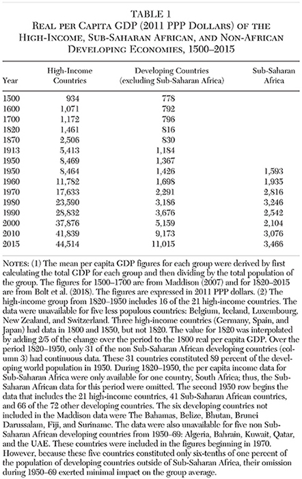
Around 1800, however, the Industrial Revolution began to transform the world. This was certainly true for the 12 to 15 percent of the world’s population living in the West and Japan. As Table 1 shows, per capita GDP in these areas rose from $1,461 in 1820 to $2,506 in 1870 and $5,413 in 1913. By 1950, the per capita GDP in these regions had soared to $8,469, an increase of 480 percent in 130 years.
But the change was much less transformative elsewhere. During the 130 years from 1820 to 1950, per capita GDP of the developing countries outside of Sub-Saharan Africa rose from $816 to $1,367, an increase of only 68 percent — less than a half of a percent annually. Moreover, the $1,367 per capita GDP of these countries in 1950 was even lower than the $1,461 per capita income of the high-income countries in 1820. These figures show that while the Industrial Revolution triggered growth in the West, its impact on the 85 percent of the population living elsewhere in the world was minimal. People in these countries did a little better during this period than prior to 1800, but not much.
The situation has changed dramatically during the past half century, first for developing countries outside of Sub-Saharan Africa and more recently for Sub-Saharan Africa (Sala-i-Martin and Pinkovskiy 2010). As Table 1 shows, per capita GDP of the developing countries outside of Sub-Saharan Africa rose from $1,698 in 1960 to $11,015 in 2015, a whopping increase of 549 percent. This increase in just 55 years was even larger than the increase in per capita GDP of the high-income countries during the 130 years following 1820. Moreover, there are signs of change in Africa. The per capita GDP of Sub-Saharan African countries has increased from $2,104 in 2000 to $3,466 in 2015, an increase of 65 percent in 15 years.
What accounts for the increased growth of the past half century? Why has per capita income in some countries grown rapidly, but lagged behind in others? How have differences in geography, institutions, international trade, and demographic changes influenced development during recent decades? This article will examine each of these questions.
The Transportation-Communication Revolution: What It Is and Why It Has Changed the Pattern of Development
Since the 1950s, there has been a huge reduction in transportation and communication costs, driven by improvements in technology and entrepreneurship. The jet engine substantially reduced the cost of both air travel and shipment of cargo. The integrated circuit and the microprocessor have improved the quality and reduced the cost of products ranging from cell phones to airplanes. The internet has vastly reduced the cost and increased the speed of transmitting information.
Consider the impact of the steel container, a low tech and largely unheralded invention. Because these containers are standardized in size and design, thousands of them can be stacked on large ships and transported at a low cost to ports throughout the world. Upon arrival, machines can lift them onto rail cars and trucks for transport to inland distribution centers and manufacturing facilities. The use of these containers has reduced the costs of loading and unloading ocean freighter cargo in the United States from $48 per ton in 1956 to 18 cents2 in 2006, a reduction of 99 percent (Hammond 2019).3 Of course, this is merely the cost of loading and unloading, not the total cost of shipping. However, until recent decades, the loading and unloading costs were a major component of total shipping costs, particularly for short and medium distance hauls.
The cost of air passenger transport has also declined sharply and the volume of international travel soared in recent decades. According to data from The World Tourism Organization, 524 million people traveled from one country to another in 1995, but that figure expanded to 1.3 billion in 2017, a whopping 148 percent increase in 22 years.4 The growth of international travel by persons from developing countries was even greater. In upper-middle-income countries, 104 million people traveled via air to a foreign country in 1995, but that figure soared to 348 million in 2017, an increase of 235 percent. For lower-middle-income countries, the increase in international air travel was even larger, going from 29 million in 1995 to 138 million in 2017 — an increase of 376 percent in just 22 years (World Bank Databank 2019).
The timing and financial cost reductions for several forms of communication have been so dramatic they are difficult to even estimate. As recently as 1980, international telephone calls were of uncertain quality and cost several dollars per minute. Today, calls involving both audio and video transmission, including conference calls, can be made over the internet at a small fraction of their cost just a few decades ago. In the 1980s, sending documents and written messages would have cost tens of dollars and the delivery taken seven days or more. Today, digital documents can be delivered in seconds at a near zero price.
Data on shipping of cargo via ocean and air provide insight on the magnitude of the changes in shipping costs. Ocean shipping constitutes 99 percent of world trade by weight and a majority by value. Figure 1, Panel A, presents the data for ocean shipping costs expressed as an ad valorem rate (the total shipping cost divided by the total value of the cargo shipped). Two series are shown in Panel A. The first is from the classic study by Hummels (2007) based on the cost and value of all imports entering U.S. ports by ship each year during 1974–2004. The second series covers 1995–2016 and is constructed using data from the OECD (2019). It is the cost of transportation and insurance as a share of the overall value of the imported shipment.5 The data series used here is a trade weighted average of U.S. shipping costs from Miao and Attia (2018). These two data series are constructed using slightly different definitions of costs, meaning that in the overlapping years (1995–2004), values are unlikely to be identical between both sets. However, both reflect dramatic changes in the cost of ocean shipping through time. Hummels’s data (2007) indicate that ocean shipping costs fell from 10 percent of the value of the shipment in 1974 to 5.8 percent in 2004, a reduction of 42 percent over these three decades.6 The OECD data indicate that ocean shipping costs, including insurance, declined from 4.2 percent of cargo value in 1995 to 2.8 percent in 2016, a reduction of 33 percent during the 21 years. Together, the two series imply that real ocean shipping costs declined by slightly more than 50 percent during 1974–2016.
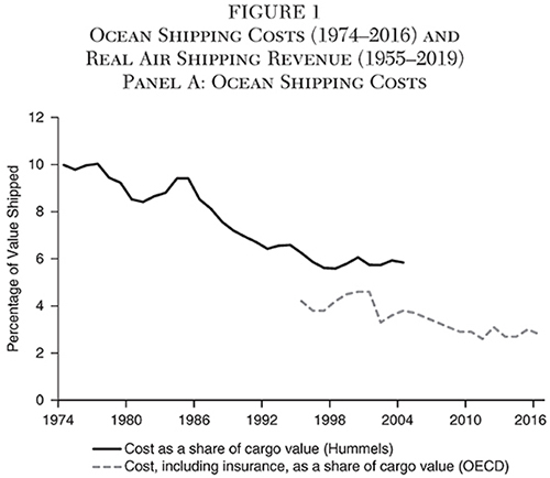
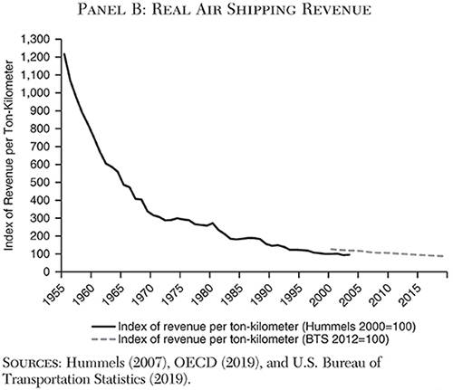
Figure 1, Panel B presents data on shipping costs via air freight. As in the case of Panel A, two series are presented. While both are based on the revenue of air carriers per ton-kilometer shipped, they cover different time spans and air carriers. The first series (Hummels 2007) is an index of the revenue per ton-kilometer shipped for all international carriers during 1955–2003. The second series (U.S. Bureau of Transportation Statistics 2019) covers 2000–19, but is only for U.S. carriers on international cargo flights. Each series is an index reflecting the real revenue earned by air carriers in U.S. dollars. The Hummels series has an index value of 100 in 2000, while the BTS series has an index value of 100 in 2012. The decline in air transport costs over the period was quite dramatic. Hummels’s data indicate that the index of air cargo shipping revenue fell from 1,217 in 1955 to 95 in 2003, a 92 percent reduction during this time span. The BTS index of revenue per ton-kilometer fell from 126 in 2000 to 87 in 2019, a 31 percent reduction during the two decades. Using the last year in which the two series overlap, the overall percentage decline of revenue per ton-kilometer for air transport during 1955–2019 was a whopping 94 percent. While a substantial share of the decline in the cost of air shipping occurred prior to 1970, the reduction during 1970–2019 was still huge — 78 percent.
The Transportation-Communication Revolution and Economic Development
There are four reasons why these reductions in transportation and communication costs will promote development: (1) gains from reductions in transaction costs and expansion in international trade; (2) increased gains from entrepreneurship and adoption of technology and successful business practices from other countries; (3) improved economic institutions; and (4) a virtuous cycle of development. Let’s take a closer look at each of these sources of growth.
First, as the reductions in transportation and communication costs increase the volume of international trade, gains from specialization and adoption of mass production techniques will increase. As a result, it will be possible for the trading partners to achieve lower costs, larger outputs, and higher income levels. In a dynamic sense, these factors will enhance economic growth.
Second, the advanced technologies and successful business practices employed in other countries are an important source of gains from entrepreneurship and improvements in productivity. This factor is particularly important in developing countries. Businesses and entrepreneurs in developing countries can merely copy (or adopt at a low cost) the successful technologies and practices of the more advanced economies. However, in order to do so, they need to know about them. The reductions in transportation and communication costs and accompanying increased interaction among people living in high- and low-income countries will provide valuable information that will accelerate this process. So, too, will the ease of accessing and transmitting information and communicating with others throughout the world.
Third, the lower transportation and communication costs will also increase the incentive to adopt economic policies more consistent with growth and development. For example, when the cost of shipping goods to major markets or obtaining resources from distant locations is high, the incentive to remove various trade barriers is weak, particularly in countries located distant from major markets. However, lower transportation costs will provide greater access to a broader set of markets, increasing the potential gains derived from reductions in trade barriers. In turn, the larger potential gains will increase the incentive of businesses and entrepreneurs to bring additional pressure for trade liberalization.
Reductions in transportation and communication costs will also influence the incentive to support a legal structure protective of property rights and enforcement of contracts. Foreign businesses and investors will be reluctant to engage in business activities when the country’s legal system fails to provide for security of property rights and enforcement of contracts. If high transportation costs make the country an unattractive place to do business, the gains derived from improvements in the legal system will be small. However, when reductions in transportation and communication costs increase the attractiveness of a country to potential businesses and investors, the gains derived from improvements in the legal system will increase, enhancing the incentive to move toward legal system improvements. Thus, in addition to their more direct impact on the volume of trade and entrepreneurship, lower transportation and communication costs will generate a positive secondary effect: enhancing incentives for countries to remove trade barriers and improve their legal systems.
Fourth, once the growth process begins, countries experience a virtuous cycle of economic development. Higher income levels increase the opportunity cost of having children and increase incentives for individuals to improve their education and skill level. As a result, the birthrate declines, leading to a reduction in the share of population within the youngest age categories and an increase in the population share within the prime working-age group. In turn, this expansion in the share of population within the prime working-age category propels additional growth. Moreover, the declining share of children and higher earnings both increase the incentive to invest in additional schooling and improve human capital, which eventually leads to still higher worker productivity and income levels.
International Trade and Economic Growth
Since the time of Adam Smith, most economists have argued that international trade facilitates higher income levels and more rapid growth. In recent years, this view has increasingly come under attack from political leaders and even a few economists. The substantial reductions in transportation and communication costs in recent years serve as a natural experiment on the relationship between increases in international trade and economic growth. Like reductions in tariffs and removal of other trade barriers, lower transportation and communication costs will increase the volume of mutually advantageous exchanges. In turn, economic theory indicates these exchanges will make it possible for the trading partners to achieve higher income levels.
If the above economic view of trade is correct, today’s expansion in trade should be associated with higher rates of economic growth. Further, countries with larger expansions in trade volume should grow more rapidly. While the relationship between international trade and economic growth is not the primary focus of our research, our empirical analysis nonetheless provides evidence on this issue. We will return to this topic over the course of this article.
The Transportation-Communication Revolution and the Pattern of Development
What impact has the reduction in transportation and communication costs had on the pattern of development in recent decades? In order to examine this question, we assembled data on per capita GDP, demographics, and economic institutions. There are 134 countries for which per capita GDP data are available from the Penn World Table version 9.1 (Feenstra, Inklaar, and Timmer 2015) continuously since 1970 for which the economic freedom of the world (EFW) (Gwartney et al. 2018) data are also available in 2015.7 This set of 134 countries constitutes the primary database of this study. In 2017, the population of these countries comprised 94 percent of the total for the world.8 Demographic data on population by age group are also available for these 134 countries for 1960–2015 (World Bank, 2019). While economic freedom data are unavailable for many of these countries for earlier years, the EFW data are available for approximately 100 countries dating back to 1980. Thus, our cross-country analysis will generally involve between 100 and 134 countries.
We divided the 134 countries in our primary database into three subgroups: (1) the 21 high-income countries of Western Europe, North America, and Oceania plus Japan; (2) 40 countries that face major geographic disadvantages as the result of their unfavorable location and climate; and (3) 73 other developing countries. Following Jeffrey Sachs (2003), we measured geographic disadvantages based on a country’s distance from major markets, malaria ecology, and proportion of population residing within 100 kilometers of an ice-free ocean coastline. Our variable for measuring distance to major markets is the minimum air distance, in thousands of kilometers, from the capital city of each country to New York, Rotterdam, or Tokyo. Malaria ecology is a purely climatological variable indicating the ecological conditions for the prevalence of malaria. The basic formula for malaria ecology includes temperature, mosquito species abundance, and specificity of mosquito vector types that are most dangerous to humans. This index ranges from zero (least dangerous) to 31 (most dangerous) environment for malaria. The ocean coastline variable, which ranges from zero to one, indicates the fraction of a nation’s population in 1994 living within 100 kilometers of an ocean coastline. The geographic disadvantage variables are from Gallup, Sachs, and Mellinger (1999) and Sachs (2003).
We standardized and added the original values of the above three geographic disadvantage variables to provide an aggregate measure for each country’s geographic disadvantage. We also standardized this aggregate measure to derive a summary geographic disadvantage measure with a zero mean and standard deviation of 1 for the 134 countries of our primary data base. Table 2 (columns 1, 2, and 3) shows the original values of the three geographic disadvantage variables for the 40 most disadvantaged countries in our analysis. Column 4 shows the summary geographic disadvantage measure, in standardized units, for each of these countries.
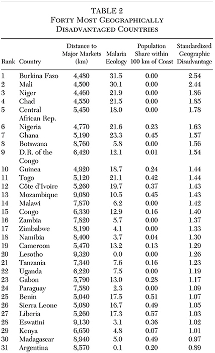
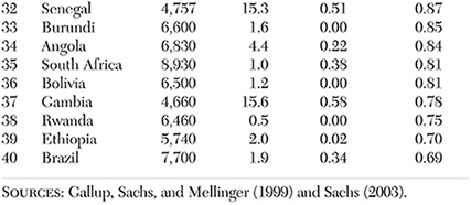
As Table 2 shows, the five most geographically disadvantaged countries are Burkina Faso, Mali, Niger, Chad, and Central African Republic. These five countries have high malaria ecology (20 or above) and are located approximately 5,000 kilometers (about 3,000 miles) from their closest major world market center (Rotterdam, New York, or Tokyo). Moreover, all five are landlocked with zero percent of their population residing within 100 kilometers of an ocean coastline. The standardized summary measure indicates these five countries confront unfavorable geographic conditions that are between 1.78 and 2.54 standard deviations from the world sample mean. Thirty-six of the 40 most geographically disadvantaged countries are Sub-Saharan African. The four exceptions are Latin American countries: Paraguay, Argentina, Bolivia, and Brazil. Among the 30 most geographically disadvantaged countries, all are Sub-Saharan African aside from Paraguay. Clearly, Sub-Saharan Africa dominates the list of countries with the most unfavorable geographic conditions.
Expansion in International Trade and the Impact of Geography
Using the Penn World Table merchandise trade data, Figure 2 shows the path of international trade as a share of GDP for the world during 1960–2017 (left axis) and the 15-year moving average of annual real per capita GDP growth during 1950–2017 (right axis).9 The growth figures are from the Maddison dataset (Bolt et al. 2018) because these data are more complete than the Penn World Table data for the years prior to 1970. During 1960–2017, international trade increased persistently and substantially as a share of global output. During the 1960s, the trade/GDP ratio averaged 19 percent of world GDP. By 1970, the ratio had risen to 20 percent, and by 1990, it was at 32 percent. It continued to rise, reaching 43 percent in 2000 and 50 percent in 2010. Since 2010, the ratio has fluctuated around 50 percent. Thus, international trade as a share of world GDP in recent years has been approximately 2.5 times the level of the 1960s.
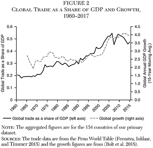
The 15-year average annual growth rate for the world, in terms of per capita GDP (shown in Figure 2), indicates that the expansion of international trade is associated with increasing growth of worldwide real per capita GDP. Prior to the early 1990s, the average growth rate of worldwide per capita GDP fluctuated between 1.9 and 2.9 percent. After 1990, as the volume of trade rose from 30 percent of global GDP to 50 percent, the 15-year moving average of global per capita GDP growth steadily increased, reaching 4.1 percent in 2015. The expansion in international trade and increased economic growth during the half century following 1965 is remarkable. However, this is precisely the expected response to such a huge reduction in transportation and communication costs.
While Figure 2 shows the aggregate expansion in merchandise trade, Figure 3 illustrates the breakdown of that expansion for each of the groups in our dataset: the 21 high-income, 40 most geographically disadvantaged, and 73 other developing countries between 1960–2017. We computed the total real value of trade (measured in 2011 dollars) for each group and transformed it into an index with a base value of 100 in 1960. Thus, changes in the index illustrate the magnitude of the change in the real value of trade for each group during the period.
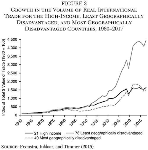
The increases in trade were most dramatic among the less geographically disadvantaged developing countries. From 1960–90, the index rose to 557 for the high-income countries, 545 for the less disadvantaged developing countries, and 282 for the geographically disadvantaged countries. This indicates that the volume of international trade in 1990 of the first two groups was approximately 5.5 times its level in 1960, while the parallel figure was only 2.8 for the geographically disadvantaged countries. After 1990, however, the growth of international trade soared for the less geographically disadvantaged developing countries and by 2017 had increased to 4,450, indicating that the total real value of trade for these countries was 44.5 times its level in 1960. This dwarfs the expansion in international trade for the other two groups: by 2017, the indices for the high-income countries and the geographically disadvantaged countries were 1,637 and 1,505, respectively. Thus, the 2017 volume of international trade of these two groups was about 15 or 16 times their level of 1960, far less than the parallel figure of 44.5 times for the less geographically disadvantaged group.
In 1960, global trade was dominated by the high-income countries. Their share of global trade stood at 69.4 percent, while the share of global trade for the less geographically disadvantaged developing countries was 24.8 percent. However, by 2017, the share of global trade for the high-income countries and less disadvantaged developing countries was approximately the same: 47.5 percent and 48.8 percent, respectively.10
Figure 4 shows the per capita real dollar value (in 2011 dollars) of international merchandise trade for the three groups. Unsurprisingly, the per capita dollar value of the trade volume of the 21 high-income countries was much larger than it was for either of the developing groups. From 1960–75, the per capita international trade of the high-income group increased substantially compared to the other countries, and in 1975 reached $5,547, more than eight times the $659 figure for each of the developing groups. Between 1960 and 1975, the per capita dollar value of trade for the 40 most geographically disadvantaged countries was generally greater than the parallel figure for the 73 developing countries.
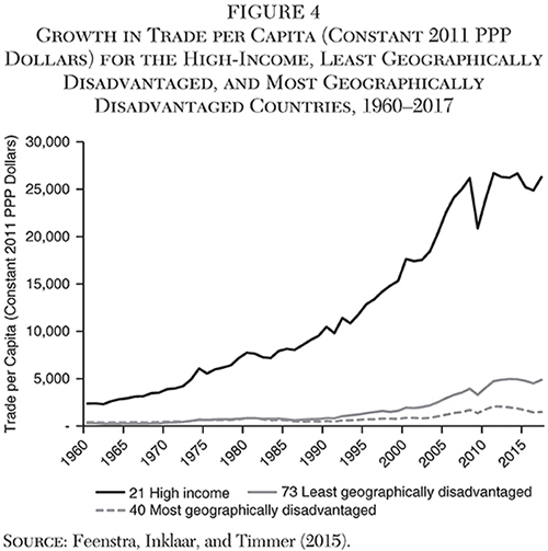
Following 1975, however, the expansion in merchandise trade for less geographically disadvantaged developing countries grew far more rapidly than it did for the geographically disadvantaged countries. By 2000, the per capita dollar value of international trade for the former group had risen to $1,936, while the same figure had risen to only $880 for the geographically disadvantaged group. The trend continued during 2000–17. By 2017, the real dollar value of international trade per capita of the least geographically disadvantaged developing countries had risen to $4,878, compared to $1,483 for the most geographically disadvantaged group. Thus, while per capita trade for both groups was equal in 1975, by 2017, the trade volume of the nongeographically disadvantaged developing countries was 3.3 times the trade volume of the geographically disadvantaged group. During 1975–2017, the per capita trade volume of the high-income countries rose from $5,547 to $26,273, an increase of 373 percent over 42 years. During this same time frame, the per capita trade for the less geographically disadvantaged developing countries rose from $649 to $4,878, an increase of 651 percent. Thus, the per capita real dollar value of international trade of the 73 developing countries rose by a substantially higher percentage than the parallel figure for the other two groups.
In summary, the volume of international trade rose substantially during the past half century (Figure 2). But the growth of international trade differs substantially across country groups. The percentage increase in the real dollar value of international trade has been far greater for the 73 developing countries than for the 21 high-income and 40 most geographically disadvantaged countries (Figure 3). Moreover, as Figure 4 shows, the dollar value of per capita international trade is much smaller for both developing groups (particularly the geographically disadvantaged group) than it is within the high-income countries. No doubt the developing countries’ substantially smaller trade volume is a major reason for their low income levels relative to their high-income counterparts.
Gains from Improvements in Economic Institutions
The reduction in transportation and communication costs will enhance incentives for developing countries to improve their economic institutions. Table 3 presents the simple mean (Panel A) and population weighted mean (Panel B) ratings for the summary economic freedom and freedom of international exchange (Area 4) using the Fraser Institute’s economic freedom of the world (EFW) data for 1985, 2000, and 2015 for the high-income and developing country groups (Gwartney et al. 2018). As expected, the ratings of the high-income group were greater than those of the developing countries. In 2017, the simple mean of the EFW summary rating for the high-income countries was 7.7, compared to 6.9 for the developing countries and 6.1 for the geographically disadvantaged countries.
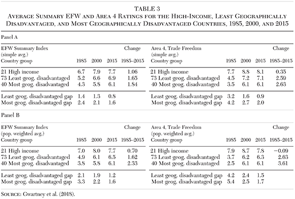
The EFW summary ratings generally rose during 1985–2015, but the increases for the developing countries were greater. Thus, the gap between the high-income and the developing groups’ EFW ratings narrowed. In 1985, the simple mean EFW summary rating of the high-income countries was 1.4 units greater than it was for the 73 developing countries and 2.4 units greater than for the 40 most disadvantaged countries. By 2015, however, this gap had fallen to 0.8 for the other developing countries and 1.6 for the geographically disadvantaged countries. In the case of the population weighted means (Panel B), the gap between the high-income and developing countries followed a similar path.
Turning to the Area 4 trade openness variable, the simple mean rating of the high-income countries was 7.7 in 1985, compared to only 4.5 for the less geographically disadvantaged developing countries and 3.5 for the most geographically disadvantaged group. In 2015, the trade openness simple mean rating of the high-income countries was 8.1, slightly higher than it was in 1985. In contrast, the simple mean ratings for the less geographically disadvantaged developing countries rose sharply during 1985–2015, narrowing the gap in trade openness between the developing and high-income countries. The gap in the simple mean between the high-income and 73 developing countries fell sharply, from 3.2 in 1985 to only 0.9 in 2015. In the case of the most geographically disadvantaged countries, the simple mean gap fell from 4.2 in 1985 to 2.0 in 2015. As Panel B shows, the population weighted mean trade openness gap between the high-income and developing countries followed a similar path. Thus, as incentive structures changed following the reduction in transportation and communication costs, the developing countries moved toward better economic institutions and more open trade.
Gains from the Virtuous Cycle of Development
Once the growth process begins, the virtuous cycle of development indicates that birth rates will decline and the share of population in the most productive age groups will rise. Thus, as reductions in transportation and communication costs, increases in gains from trade, and improvements in economic institutions ignite the growth process, increases in the share of population in the prime working-age categories will further boost economic growth. Of course, higher rates of economic growth will accelerate this process, causing the share of population in the prime working-age categories to increase rapidly.
Figure 5 shows the share of the population within the prime working-age category (ages 25–59), relative to the total, for each of our three major groups since 1950. During 1950–70, the prime working-age share of the population trended downward across all three groups. This worldwide trend reflected the dearth of births during the economic hardship of the Great Depression and World War II and the substantial increase in the birth rate following the postwar boom.
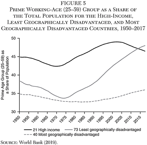
The share of the prime working-age population within the high-income countries rose by approximately 2 percentage points per decade during 1970–2000, but it has declined at a similar rate since the onset of the 21st century. In 2017, the prime working-age group comprised 46.5 percent of the total population of the high-income countries, down from 49 percent in 2000. The prime working-age share of the population for the 73 less geographically disadvantaged developing countries was much lower than it was for the high-income countries during the 1970s, but this situation changed dramatically over the next four decades. The prime working-age share of the population for the less geographically disadvantaged developing countries rose from 34 percent in 1975 to 38 percent in 1990, before soaring to 46 percent in 2010. During 1990–2010, the prime working-age share of this group’s population increased by a whopping 4 percentage points per decade. By 2017, the prime working-age share of the population was higher for these 73 developing countries (48 percent) than it was for the high-income group (46.5 percent).
Compared to the other two groups, the prime working-age share of the population for the most geographically disadvantaged countries was substantially lower and increased at a slower rate during the past half century. The prime working-age share of the population for the most geographically disadvantaged group fluctuated within a narrow band (around 33 percent) between 1970–90, before trending slowly upward to 36 percent in 2017. In 2017, the prime working-age share of the population for the most geographically disadvantaged countries was more than 10 percentage points below the parallel figures for the other two groups.
The virtuous cycle of development implies that these differences in demographic changes impact the pattern of economic growth for each of the three groups. The expansion in the share of population in the high-productivity, prime working-age category for the high-income countries during 1970–2000 and the less geographically disadvantaged developing countries during 1975–2017 tended to enhance their economic growth. On the other hand, the low and more stable prime working-age share of the population in the most geographically disadvantaged countries tended to adversely affect their growth and development.
International Trade, Institutions, Demography, and the Pattern of Development during the Past Half Century
As would be expected, the huge reductions in transportation and communication costs of the Transportation-Communication Revolution substantially increased the volume of international trade, particularly for the less geographically disadvantaged countries we studied. Improvements in the economic institutions and policies of developing countries, as well as demographic changes (the share of population in the prime working-age category), have also accompanied the Transportation-Communication Revolution. How important are these factors as sources of economic growth?
Prior research utilizes cross-country differences in both trade policy and volume to examine the impact of trade on economic performance. Various measures of trade policy, including composite trade openness indices, tariff rates, and black market exchange rates have been employed (Sachs and Warner 1995; Edwards 1998). This research generally finds a positive relationship between more open trade policies and higher rates of economic growth. However, relying only on the above measures is problematic as they do not adequately capture all aspects of trade policy (Rodríguez and Rodrik 2001). Moreover, the trade policy research suffers from two additional shortcomings. First, countries with more open trade policies also generally have better institutions (e.g., legal structure, regulatory policy, and constraints on the executive). This makes it difficult to determine the importance of trade policy relative to other institutional factors. Second, geography influences the impact of trade policy on economic growth. For example, the impact of a reduction in tariff rates will be very different for countries like Ireland and Hong Kong, which are located near major markets, than for countries like Uganda and the Central African Republic, which are landlocked and distant from major markets. Past research on the impact of trade policy generally fails to account for these factors.
Additional research has focused on how variations in the size of the trade sector influence economic growth (Frankel and Romer 1999; Yanikkaya 2003). The volume of international trade as a share of GDP has generally been used to measure the size of the trade sector. Unfortunately, there are problems with this measure as well. Trade as a share of GDP varies substantially according to both country population and area. International trade as a share of GDP will be larger for smaller, less populous countries than it will be for their larger counterparts. Moreover, countries with larger trade sectors often also have superior economic and political institutions, leading to multicollinearity between international trade and institutional quality (Dollar and Kraay 2003). These methodological shortcomings weaken confidence in the findings of prior research.
Our analysis measures the expansion in the size of a country’s trade sector using the change in the real volume of international trade over three 15-year periods and one 12-year period, divided by the GDP in the first year of each period. This variable measures the magnitude of changes in the relative volume of trade during a period regardless of a country’s size, level of development, or geographic characteristics. It is important to consider growth over a lengthy time frame because, during short periods, a country’s growth rate will be affected by random shocks, phases of the business cycle, and similar temporary factors. Moreover, it will take time for changes in technology, shipping costs, and policy to exert an impact on the volume of trade and economic growth. Thus, our analysis examines the impact of changes in the volume of trade, as well as institutional and demographic factors, on economic growth over lengthy time periods.
Regression Results
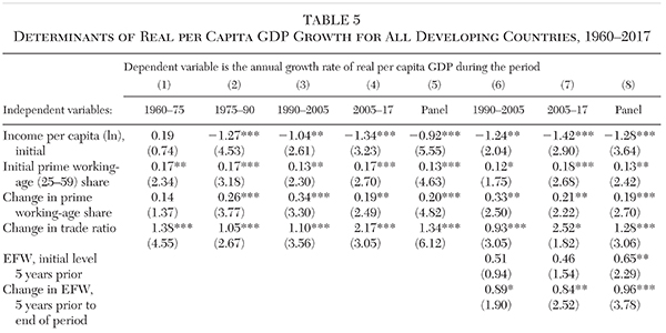
Table 4 shows the regression equations for our growth model with the annual growth rate of real per capita GDP (in 2011 dollars) as the dependent variable. Changes in the volume of international trade, share of the population in the prime working-age category, and economic freedom are included as independent variables, along with a set of control variables. The trade variable is the change in international trade in real 2011 dollars during each period divided by real GDP at the beginning of the period. A one unit increase in this variable indicates that the increase in real international trade (exports 1 imports) during that period is equal to the initial real GDP. Both the share of population in the prime working-age category (ages 25–59) at the beginning of each period and the change in that share during the same period are also included as independent variables. Similarly, the level of economic freedom five years prior to the beginning of each period and change through the end of the period are incorporated as measures of economic institutions. Theory indicates that each of these variables will have a positive impact on the growth of real GDP per capita.
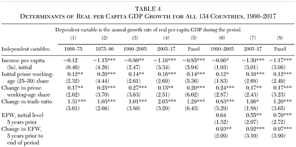
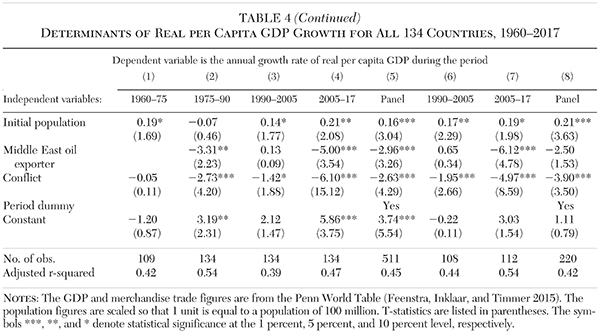
Four control variables are also included in our model: log of per capita GDP; population; and two dummy variables. The log of per capita GDP at the beginning of each time period is designed to reflect a country’s initial stage of development. If lower income countries are growing more rapidly than their high-income counterparts, this variable will be negative. This is often the case because low-income countries are able to copy (or acquire at a low cost) successful technologies and business practices of high-income countries. The reduction in transportation and communication costs of recent decades amplifies the importance of this factor. Population (in hundreds of millions), our second control variable, is expected to generally be positive because populous countries have larger domestic markets, which will result in larger gains from both the adoption of mass production processes and increased attractiveness to foreign investors. We included a dummy variable for countries experiencing conflicts resulting in more than one fatality per thousand during any of the last five years of a period. Since war and other forms of bloody conflict generally adversely impact economic growth, this variable is expected to have a negative sign. Finally, we included a dummy variable for six small middle eastern oil exporters (United Arab Emirates, Qatar, Bahrain, Kuwait, Oman, and Saudi Arabia). Somewhat paradoxically, the per capita GDP of these countries often declines during periods of high and rising oil prices because of increased inflows of immigrant workers with incomes well below the national average. Thus, this variable is expected to be negative, particularly when world oil prices are high.
We ran our model over four time frames: 1960–75, 1975–90, 1990–2005, and 2005–17. Since economic freedom data are only available for a large set of countries during the last two periods, columns 1 through 4 represent the results of our model without its economic freedom variable, while columns 6 and 7 represent results using our full model. Columns 5 and 8 present the results of our panel analysis for the first four and final two periods, respectively.
As Table 4 shows, the change in the size of the trade sector was positive and significant at the 1 percent level for all equations except for equation 7 (where it was significant at the 10 percent level). The coefficient of the trade variable in the first three equations ranged from 1.01 to 1.31, indicating that, after adjusting for the other variables, a one unit expansion in the size of the trade sector during each period was associated with a higher annual growth rate of 1 to 1.3 percentage points. Note: the size of the trade coefficient during 2005–17 was even larger, approximately 2 (column 4), consistent with the view that the impact of international trade on growth was strongest during the most recent period. As column 3 shows, the coefficient on the trade variable during 1990–2005 was 1.01, implying that a one unit increase in the size of the trade sector during this 15-year period was associated with an annual growth rate increase of 1.01 percentage points. Consider the following example: the value of the trade sector variable for Argentina, Ecuador, and Romania was approximately 0.5 during 1990–2005, compared to 1.5 for Norway and Jordan. This suggests that, after adjusting for the impact of the other variables, additional trade enhanced the annual growth rate of the latter two countries, relative to the former, by about 1 percentage point.
Both the prime working-age population as a share of the total and the change in that share (during each period) were positive and significant in all equations, generally at the 5 percent level or higher. The coefficient for the change in prime working-age population was approximately 0.2, indicating that a one percentage point expansion in the prime working-age share of the population was associated with a 0.2 percentage point increase in the annual growth of per capita GDP during each period.
Our control variables generally performed as expected. The pattern of the per capita GDP at the beginning of each period was particularly interesting: the initial GDP variable was insignificant during 1960–75 but negative and significant for the last three periods. The negative sign indicates convergence — the countries with lower initial per capita GDP grew more rapidly than their higher income counterparts for periods beginning after 1975.
Columns 6, 7, and 8 integrate our economic freedom variable into the analysis. The level of economic freedom was generally positive and significant. The change in economic freedom during the past 20 years (17 in the case of the last period) was always significant at the 5 percent level or higher. The coefficients for the change in economic freedom variable ranged from 0.92 to 0.97, indicating that each unit increase in economic freedom during any given period increased that period’s annual growth rate by slightly less than 1 percentage point.
Panel data methods provide more precise estimates of the relationship between our independent variables and the dependent variable, primarily because of the increased number of observations. Column 5 presents the pooled OLS panel results of the model without the economic freedom variable and column 8 shows the results with the economic freedom variable. In our panel analysis, the coefficients of these variables are similar to those for each individual period and their significance levels are generally higher. In our panel analysis, the coefficients for the trade variable were 1.29 (column 5) and 1.20 (column 8). This indicates that a one unit increase in the international trade variable is associated with an estimated 1.2 to 1.3 percentage point increase in the annual growth rate of real per capita GDP. In the panel analysis, the coefficients for the change in the prime working-age population variable were 0.20 and 0.17, respectively. This implies that a percentage point increase in the share of population in the prime working-age category enhances the annual growth rate of per capita GDP by approximately two-tenths of a percentage point. The coefficient for the change in economic freedom in our panel analysis (column 8) was 0.97, indicating that a one unit increase in economic freedom enhances economic growth by nearly a percentage point. These three key variables were positive and significant at the one percent level in the panel analysis. As the adjusted r‑square indicates, the explanatory power of the model was high — 45 and 42 percent for columns 5 and 8, respectively. Lastly, the panel analysis includes dummy variables in order to control for period effects across time.
Robustness Checks
In order to examine robustness, the model was run for a different set of countries, different time periods, and with alternative measures of GDP and trade. It is important to determine if the results are affected by the inclusion of the high-income countries. Therefore, Table 5 includes only developing countries in the regressions; the 21 high-income countries are omitted.
As in Table 4, the dependent variable in Table 5 is the annual growth rate of real per capita GDP. The independent variables are also identical. Even though the high-income countries were omitted from the version of the model used for Table 5, the results are similar to those of Table 4. Once again, the variables for international trade, change in the prime working-age share of the population, and economic freedom were highly significant. The coefficients of the international trade variable in the panel analysis (columns 5 and 8) were 1.34 and 1.28, respectively, indicating that a one unit increase in the trade variable increases the annual growth rate by an estimated 1.3 percentage points. This is virtually the same as the estimates of Table 4. Both the level and change in the share of population in the prime working-age category were highly significant. The coefficients in the panel regressions indicate that a one percentage point increase in the share of population in the prime working-age category increases the annual growth rate by approximately two-tenths of a percentage point. Again, the coefficient for the change in economic freedom (0.96 in the panel analysis) indicates that a one unit change is associated with a little less than a percentage point increase in the annual growth rate of real per capita GDP. The control variables and explanatory power of the model are virtually unchanged from the results of Table 4. These findings show that the trade, demographic, and economic freedom variables continue to exert a strong impact on economic growth when only developing countries are included in the analysis.
Table 6 is similar to Table 4 except the time periods differ. Table 6 shows the results of the model for three alternative 15-year periods: 1970–85, 1985–2000, and 2000–15. Again, the dependent variable is the annual growth rate of real per capita GDP during each period. The results show that our model is highly stable across varying time periods. The coefficients of the trade variable (1.05 and 0.88 in the panel analysis, columns 4 and 7) are slightly lower than those of Tables 4 and 5. However, these coefficients are actually a little more significant than they are in the prior analysis. Here, the t‑ratios for the trade variable coefficients are exceedingly high — 9.39 in the first panel regression, and 4.65 in the second. The coefficients on the change in the prime working-age share of the population were 0.20 and 0.24 in the two panel regressions, once again indicating that a percentage point increase in the share of population in the prime working-age group is associated with approximately two-tenths of a percentage point increase in the annual growth rate of real per capita GDP. The 1.0 coefficient for the change in economic freedom implies that a unit change in this variable enhances the annual growth rate by approximately one percentage point. The pattern of the control variables is also similar to that of the prior analysis. The r‑squares for Table 6’s panel equations (0.46 and 0.52) are a little higher than in Table 4, indicating a slight increase in the explanatory power of the model.
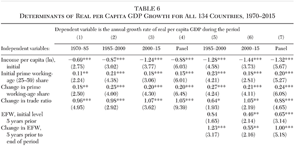
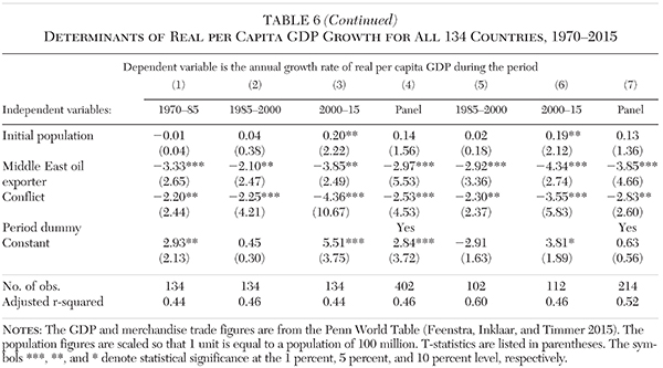
Table 7 replaces the Penn World Table measures of GDP and international trade in 2011 purchasing power parity dollars with the World Bank measures. In addition, the trade measure is now for goods and services, rather than merchandise trade. The broader trade measure that includes services is unavailable from the Penn World Table data set. A disadvantage of using the World Bank data is that the GDP and trade data in constant PPP 2011 dollars are unavailable for years prior to 1990. Thus, Table 7 covers only two time periods: 1990–2005 and 2005–17. Further, the overall number of observations is slightly lower (116 and 127 rather than 134) because the World Bank data were unavailable for a few of the 134 countries in our data set.
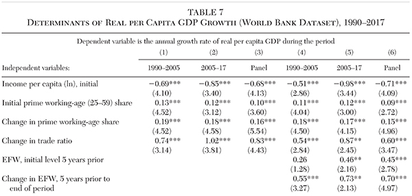
In spite of these differences, the results are similar to those derived using the Penn World Table data. As in the prior analysis, the expansion in international trade, change in the prime working-age share of the population, and increase in economic freedom variables are highly significant (generally at the 1 percent level). However, their coefficients are slightly smaller. The coefficients for the expansion in international trade variable are now 0.83 and 0.60 in the Table 7 panel analysis, down from approximately 1.2 in Table 4. In the case of the prime working-age variable, the coefficients range from 0.15 to 0.19, slightly lower than the prior estimates of 0.20. The estimated impact of economic freedom on growth is 0.70, compared to the approximately 1.0 in prior tables. The r‑squares (0.49 and 0.54) in the panel analysis are slightly higher than for the Penn World Table data. The r‑squares for the full model, including economic freedom, indicate that the independent variables explain 54 percent of the cross-country variation in growth rates.
In addition to the robustness checks of Tables 5–7, other analyses were performed. The panel regressions of Table 4 were also run using a seemingly unrelated regression (SUR) model. The t‑ratios on the variables of interest were even larger than those shown in Table 4. Thus, the OLS results appear to be more conservative. In addition to SUR, the panel regressions were also run to account for fixed effects. The significance of the variables for international trade, change in the prime working-age share of the population, and economic freedom remained unchanged. We also re-ran Tables 4 and 7 with the primary trade variable expressed in per capita dollars (the change in the real value of trade per capita over the period divided by the initial real per capita GDP). Again, the results were similar and the modified trade variable remained a positive and significant predictor of economic growth. Finally, we extended the World Bank data from Table 7 back to 1985 and re-ran our model for the two periods between 1985–2000 and 2000–17. The results were virtually identical to those of Table 7.
Tables 4 through 7 illustrate that international trade, demographic changes, and economic institutions exerted a strong and consistent impact on the growth of per capita income during 1960–2017. This supplements our prior analysis showing that as the cost of transportation and communication fell sharply during the past half century, international trade expanded and became a substantially larger share of world output (Figure 2). As Figures 3 and 4 show, the trade sectors of developing countries, particularly those that are less geographically disadvantaged, grew rapidly. In addition, the lower transportation and communication costs increased incentives for developing countries to adopt policies and institutions more consistent with trade openness and economic freedom, and they responded accordingly (see Table 3). As gains from trade and movements toward economic freedom enhanced the growth of per capita GDP, the virtuous cycle of development and accompanying increase in the share of population in the prime working-age category provided an additional boost to economic growth. These factors have propelled the economic growth of less geographically disadvantaged developing countries since 1980, and there are signs that they are now accelerating the growth of even the most geographically disadvantaged countries. As a result, the world is now in the midst of an unprecedented period of development: for the first time in history, the growth of worldwide per capita income is strong and the poorer countries are growing more rapidly than their high-income counterparts.
International Trade and Economic Growth: A Natural Experiment
The sharp reductions in transportation and communication costs over the past half century provide a natural experiment on the relationship between international trade and economic growth. As our analysis shows, lower transportation and communication costs directly encourage more trade. In addition, these cost reductions increase incentives for countries to reduce their trade barriers. As a result, the volume of international trade should increase expanding the gains from specialization, economies of scale, and entrepreneurship, leading to more rapid economic growth. This is precisely what happened during the past half century: world trade increased and the worldwide growth rate of per capita GDP accelerated (see Figure 2).
Moreover, increases in international trade exerted a strong and highly significant impact on the annual growth rate of per capita GDP, even after accounting for cross-country differences in initial per capita GDP, changes in the prime working-age share of the population, economic freedom, population, and other control variables. The positive and highly significant impact of the expansion in international trade on the growth of per capita GDP was present across different time periods, for developing countries only, and for alternative measures of trade — both merchandise and goods and services trade (see Tables 4 through 7).
Unsurprisingly, the least geographically disadvantaged developing countries experienced the largest increases in international trade during the Transportation-Communication Revolution (see Figure 3). In turn, these countries have grown more rapidly than either the high-income or the more geographically disadvantaged groups over the past half century. In recent decades, the growth of the less disadvantaged developing countries has also exceeded the growth of the highest-income countries during the Industrial Revolution.
While our analysis makes no distinction between increases in international trade resulting from lower transportation and communication costs and those generated by more open trade policies, it indicates that increases in international trade have exerted a positive and highly significant impact on the growth of real per capita GDP during the past half century. These findings provide strong support for the mainstream economic view that higher rates of international trade enhance economic growth, regardless of whether those increases are generated by reduced transaction costs or more open trade policies.
The Transportation-Communication Revolution versus the Industrial Revolution
Lower transportation and communication costs have led to higher rates of integration, entrepreneurial activity, and exchange of both goods and ideas — among people living in both high- and low-income countries — than at any other time in history. The changes of the past half century have created something akin to a second Industrial Revolution: the Transportation-Communication Revolution. Like the Industrial Revolution, this more recent revolution has expanded opportunities and enhanced economic growth. But the two revolutions differ in three important respects.
First, the impact of the Transportation-Communication revolution is much broader. The Industrial Revolution resulted in substantial income gains for between 12 and 15 percent of the world’s population. However, as Table 1 indicates, its impact on the rest of the world was minimal for nearly a century and a half. In contrast, the Transportation-Communication Revolution has already exerted a major impact on approximately 70 percent of the world’s population, and its scope is still expanding.
The increasing share of world GDP generated by the 73 least geographically disadvantaged developing countries illustrates the breadth of the recent economic revolution. These countries generated 24.8 percent of world GDP in 1960, 27.8 percent in 1980, 33.3 percent in 2000, and 47.5 percent in 2017. Remarkably, during the 57 years following 1960, the share of global GDP produced in these countries has doubled.
Second, growth rates during the Transportation-Communication Revolution have been more rapid than they were during the Industrial Revolution. During 1960–2015, the real per capita GDP of developing countries outside of Sub-Saharan Africa rose by 549 percent in just 55 years, an even larger increase than that of the high-income countries during the 130 years (1820–1950) following the Industrial Revolution (see Table 1). In recent decades, almost all of the most rapidly growing economies have been those of developing countries.
Moreover, developing countries today are able to achieve growth rates beyond what was thought to be possible only a few decades ago. Prior to 1950, long-term growth rates above 2 percent were largely absent. In the 1800s, even the annual real growth rates of per capita GDP for the United Kingdom and United States — the most prosperous of the high-income economies at that time — were 1.0 percent and 1.4 percent, respectively. During the 12 decades from 1820 to 1940, the annual growth of real per capita GDP in the United Kingdom and United States exceeded 2 percent during only one decade for each country.11 These modest growth rates stand in stark contrast to those of developing countries in recent years. The annual growth rate of real per capita GDP for 44 of the 73 less geographically disadvantaged developing countries exceeded 3 percent between 2000 and 2015. Many developing countries grew even more rapidly during the past half century. Consider the following examples. The real per capita GDP of Hong Kong grew at an annual rate of 4.9 percent from 1960 to 2000. The growth rate of Singapore was even more impressive, hitting 5.7 percent during that same 40-year period. Botswana grew at an annual rate of 5.4 percent from 1965 to 2015. From 1970 to 2015, the real per capita GDP of South Korea and Indonesia grew at annual rates of 5.5 percent and 3.6 percent, respectively. Still more recently, the real per capita GDP of China rose at an annual rate of 5.9 percent between 1980 and 2015. In India, real per capita GDP rose by a rate of 4.8 percent annually between 1990 and 2015.
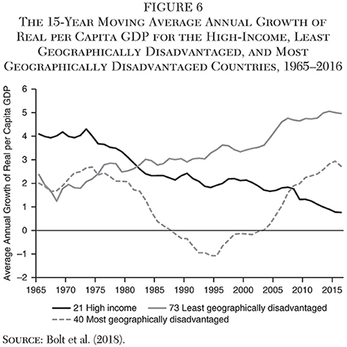
Third, while the Industrial Revolution increased income inequality, the Transportation-Communication Revolution has reduced it. Following the Industrial Revolution, income levels in the high-income countries grew, while they stagnated in the rest of the world. Thus, decade after decade, worldwide income inequality increased. In contrast, since the mid-1980s, the per capita income in developing countries, particularly those with minimal geographic disadvantages, has increased more rapidly than it has in high-income countries. Figure 6 illustrates this point. The figure shows the 15-year moving average of the growth rate of real per capita GDP for the three groups in our analysis. Prior to the mid 1980s, the high-income countries grew more rapidly than the less geographically disadvantaged developing countries. Since the mid-1980s, however, this situation has changed dramatically. Between 1985 and 2000, the average annual growth rate of the less geographically disadvantaged developing countries was 3.4 percent, compared to 2.1 percent for the high-income countries. By 2016, that growth advantage was even greater — 4.96 percent for the developing group, compared to 0.76 percent for the high-income countries. Between 2001 and 2016, even the 40 most geographically disadvantaged developing countries were achieving a solid annual growth rate (2.71 percent). As a result, worldwide income inequality has declined sharply in recent years.12
Conclusion
The Industrial Revolution transformed subsistence living into sustained growth, but only for about 15 percent of the world’s population. Throughout the rest of the world, change was minimal. In 1950, the real per capita income for developing countries outside of Africa was slightly less than $4 per day, approximately the same as that of the high-income, developed countries at the onset of the Industrial Revolution. But income levels in the developing world have increased dramatically during the past half century, particularly for the 70 percent of the world’s population living in less geographically disadvantaged developing countries.
The huge reductions in transportation and communication costs over the past half century provided the foundation for the remarkable increases in economic development and worldwide income. The Transportation-Communication Revolution triggered four changes that have altered life in the developing world: gains from large increases in international trade; gains from higher rates of entrepreneurship and expanded opportunities to borrow successful technologies and business practices from high-income countries; improvement in economic freedom; and the virtuous cycle of development.
Our empirical analysis of the annual growth rate of real per capita GDP since 1960 indicates that the expansion of international trade, higher rates of economic freedom, and increases in the share of the global population in the prime working-age category have exerted a strong and highly significant impact on economic growth. Due to the sharp reductions in transportation and communication costs, the volume of international trade has risen sharply in recent decades. The growth of trade in less geographically disadvantaged developing countries has been particularly remarkable. Measured in real dollars, the size of the international trade sector in these countries was 44 times higher in 2017 than it was in 1960. This astonishing rate of growth in international trade was approximately 2.5 times higher than it was in high-income and more geographically disadvantaged countries over the same time frame. Propelled by the growth of trade, the real per capita GDP of the five billion people living in the less geographically disadvantaged developing world has grown at nearly twice the rate of high-income countries in recent decades. The historically high rates of economic growth have transformed these developing countries even more rapidly than the Industrial Revolution transformed the West between 1820 and 1950.
While the Industrial and Transportation-Communication Revolutions exerted a similar impact on the lives of those most affected, they differ in three major respects. Compared to the earlier economic revolution, the more recent revolution has been broader, generated more rapid rates of economic growth, and reduced income inequality rather than enlarged it. Both the general populace and the academic literature show an appreciation of the human progress that accompanied the Industrial Revolution. It is now time for both groups to recognize the remarkable human progress brought about by the Transportation-Communication Revolution.
References
Bolt, J.; Inklaar, R.; de Jong, H.; and van Zanden, J. (2018) “Rebasing ‘Maddison’: New Income Comparisons and the Shape of Long-Run Economic Development.” Maddison Project Working Paper No. 10. Available at www.ggdc.net/maddison.
Dollar, D., and Kraay A. (2003) “Institutions, Trade, and Growth.” Journal of Monetary Economics 50 (1): 133–62.
Edwards, S. (1998) “Openness, Productivity, and Growth: What Do We Really Know?” Economic Journal 108 (447): 383–98.
Feenstra, R.; Inklaar, R; and Timmer, M. (2015) “The Next Generation of the Penn World Table.” American Economic Review 105 (10): 3150–82.
Frankel, J., and Romer, D. (1999) “Does Trade Cause Growth?” American Economic Review 89 (3): 379–99.
Gallup, J.; Sachs, J.; and Mellinger, A. (1999) “Geography and Economic Development.” International Regional Science Review 22 (2): 179–232.
Gwartney, J.; Connors, J.; and Montesinos, H. (2019) “The Rise and Fall of Worldwide Income Inequality, 1820–2035.” Paper presented at the Annual Meeting of the Public Choice Society (March 16). Available at http://as.nyu.edu/content/dam/nyu-as/econ/misc/Worldwide%20Income%20Inequality%201820–2035.pdf.
Gwartney, J.; Lawson, R.; Hall, J.; and Murphy, R. (2018) Economic Freedom of the World: 2018 Annual Report. Vancouver, B.C.: Fraser Institute.
Hammond, A. (2019) “Heroes of Progress, Pt. 17: Malcom McLean.” Human Progress (May). Available at https://humanprogress.org/article.php?p=1905.
Hummels, D. (2007) “Transportation Costs and International Trade in the Second Era of Globalization.” Journal of Economic Perspectives 21 (3): 131–54.
Levinson, M. (2006) The Box: How the Shipping Container Made the World Smaller and the World Economy Bigger. Princeton, N.J.: Princeton University Press.
Maddison, A. (2007) Contours of the World Economy, 1–2030 AD: Essays in Macro-Economic History. New York: Oxford University Press.
Malthus, T. (1798) An Essay on the Principle of Population. London: J. Johnson.
Miao, G., and Attia, V. (2018) “Estimating Transport and Insurance Costs of International Trade: 2018 Update.” Available at http://www.oecd.org/sdd/its/Estimating-transport-and-insurance-costs.pdf.
OECD (2019) OECD Stat. Available at https://stats.oecd.org.
Rodríguez, F., and Rodrik, D. (2001) “Trade Policy and Economic Growth: A Skeptic’s Guide to the Cross-National Evidence.” NBER Macroeconomics Annual 2000 15: 261–338.
Sachs, J. (2003) “Institutions Don’t Rule: Direct Effects of Geography on Per Capita Income.” NBER Working Paper No. 9490.
Sachs, J., and Warner, A. (1995) “Economic Reform and the Process of Global Integration.” Brookings Papers on Economic Activity 1995 (1): 1–118.
Sala-i-Martin, X., and Pinkovskiy, M. (2010) “African Poverty Is Falling Much Faster Than You Think!” NBER Working Paper No. 15775.
U.S. Bureau of the Census. (1961) Statistical Abstract of the United States: 1961. Washington: U.S. Government Printing Office.
_________ (2001) Statistical Abstract of the United States: 2001. Washington: U.S. Government Printing Office.
U.S. Bureau of Transportation Statistics (2019) U.S Air Carrier Traffic. Available at www.transtats.bts.gov/TRAFFIC.
World Bank (2019) World Development Indicators. Available at http://databank.worldbank.org/wdi.
Yanikkaya, H. (2003) “Trade Openness and Economic Growth: A Cross-Country Empirical Investigation.” Journal of Development Economics 72 (1): 57–89.
1 The 21 high-income countries that constitute the West plus Japan are Australia, Austria, Belgium, Canada, Switzerland, Germany, Denmark, Spain, Finland, France, United Kingdom, Ireland, Iceland, Italy, Japan, Luxembourg, Netherlands, Norway, New Zealand, Sweden, and the United States.
2 Both figures are in 2011 U.S. dollars; see Hammond (2019) for details.
3 See Levinson (2006) for additional details on how the development of the steel container changed the international shipping industry.
4 These data are available from the World Bank Databank (2019).
5 Specifically, the OECD series is the CIF-FOB margin — the total cost of bringing a shipment into the United States including insurance and freight (called CIF), minus the FOB value (value of the shipment not including the cost of insurance and freight) all divided by CIF.
6 The U.S. Census data on the employment of longshoremen and stevedores provides additional evidence that the use of steel containers and mechanized methods for loading and unloading substantially reduced labor costs during this same period. Even though the volume of international trade of the United States increased more than fourfold during the period, employment in this job category declined from 64,340 in 1960 to 13,550 in 2000, a 79 percent reduction during the four decades (U.S. Bureau of the Census 1961, 2001).
7 The Penn World Table data were employed because they provide real GDP and international trade data back to 1950. Later, the World Bank data will be employed to test for robustness during more recent time periods.
8 The countries formed from the former Soviet Union, Yugoslavia, and Czechoslovakia were omitted because of the absence of their data prior to the 1990s. These countries constituted two-thirds of the omitted population.
9 Merchandise trade does not include trade of services. The merchandise trade figures generally comprise about three-fourths of total international trade, including services. The data for the average growth rate begins in 1950. However, because of the 15-year moving average, the displayed data begins in 1965.
10 The World Bank provides international trade data for goods and services back to 1960. Using these data, the international trade of the nongeographically disadvantaged developing group summed to 56 percent of the world total in 2017, a slightly larger share than for merchandise trade. Moreover, the increase in the World Bank trade share for goods and services of the 73 developing countries during 1960–2017 was even larger than the increase in the merchandise trade figures of the Penn World Table.
11 The decades were, respectively, a 2.6 percent growth rate for the United States during the 1870s and 2.1 percent for the United Kingdom during the 1920s.
12 In 2015, the cross country Gini coefficient for the world was 0.466, down from a high of 0.604 in 1980. The 2015 cross-country Gini coefficient was lower than the figure in 1913 (0.495). See Gwartney, Connors, and Montesinos (2019).
About the Authors
Joseph Connors is Assistant Professor of Economics at Florida Southern College, James D. Gwartney holds the Gus A. Stavros Eminent Scholar Chair at Florida State University, and Hugo M. Montesinos is Assistant Professor of Statistics in the Department of Mathematics and Computer Science at Ursinus College.

This work is licensed under a Creative Commons Attribution-NonCommercial-ShareAlike 4.0 International License.