[The] persistent shortfall in inflation from our target has led some to question the traditional relationship between inflation and the unemployment rate, also known as the Phillips curve.… My view is that the data continue to show a relationship between the overall state of the labor market and the change in inflation over time. That connection has weakened over the past couple of decades, but it still persists, and I believe it continues to be meaningful for monetary policy.
— Fed Chairman Jerome Powell (2018: 6–7)
The history of economic thought is replete with examples of economic ideas that are politically attractive and persist even after they have little empirical support or theoretical validity. That has certainly been the case with the Phillips curve.
The Federal Reserve continues to incorporate the Phillips curve in its macroeconomic models even though the empirical evidence for a negative relationship between inflation and unemployment is weak at best. In a recent study by the Brookings Institution, the authors note that the Fed still relies on the Phillips curve as a “key factor” in setting its policy rate and as a “tool … to forecast what will happen to inflation when the unemployment rate falls, as it has in recent years” (Ng, Wessel, and Sheiner 2018: 1–2).
This article traces the history of the Phillips curve and argues that it is a poor guide for monetary policy. The underlying problem is that the Phillips curve misconstrues a supposed correlation between unemployment and inflation as a causal relation. In fact, it is changes in aggregate demand that cause changes in both unemployment and inflation. The Phillips curve continues to misinform policymakers and lead them astray.
Evolution of the Phillips Curve
In 1958, New Zealand economist A. W. Phillips published a landmark paper showing an inverse relationship between unemployment and the rate of change in money wages in the United Kingdom from 1861 to 1913. He also found that relationship persisted when the data set was extended to 1957 (Phillips 1958).
R. G. Lipsey (1960) provided further support for Phillips’s findings, as did Paul Samuelson and Robert Solow (1960), who coined the term “Phillips curve.” In their version of the curve, price inflation (rather than wage inflation) is plotted against unemployment. Using U.S. data for 1934 to 1958, they found a negative relationship between the rate of change in the average level of money prices and the level of unemployment. By viewing the Phillips curve as a “menu of choice[s] between different degrees of unemployment and price stability,” Samuelson and Solow opened the door for policymakers to believe they could fine-tune the economy by choosing a socially optimal point on the Phillips curve, at least in the short run (see Humphrey 1986:100–03).
Although Samuelson and Solow (1960: 193) stated that their analysis pertained to the short run, and that the shape of the Phillips curve could change in the long run, or the curve could shift, those caveats were largely ignored in the 1960s. There was a strong sense that the Phillips curve was stable and that there was a permanent tradeoff between inflation and unemployment. That belief fostered the idea that mild inflation was beneficial in reducing unemployment. In such an environment, inflation increased from 1.2 percent in 1962 to 5.8 percent in 1970 (see Hall and Hart 2012: 62–64).
In his monumental History of the Federal Reserve, Allan Meltzer, paints a succinct picture of the raise of the Phillips curve as a policy guide in the 1960s:
The Phillips curve was an empirical relation with no formal foundation, but it had great appeal and moved with remarkable speed from the economics journals to the policy process. Samuelson and Solow (1960) estimated the Phillips curve on data for the United States. Both worked with the new administration before the election and in its early years, Samuelson as an informal, personal adviser to President Kennedy and Solow as a senior staff member of the Council of Economic Advisers. Their paper contained a phrase about the relation of inflation to unemployment that they and others chose to ignore: “A first look at the scatter is discouraging; there are points all over the place” (ibid., 188). They recognized, however, that the shape of the curve, hence the tradeoff, depended on the policies pursued. Almost all discussion ignored the fact that most of the data which Phillips used came when the gold standard tied down expected inflation [Meltzer 2009: 268, fn.3].
In a separate study of the Samuelson-Solow Phillips curve, Hall and Hart (2012: 63–64) note:
Samuelson and Solow interpreted their statistical Phillips curve as a structural relationship that had the potential of offering a menu of exploitable tradeoffs between inflation and unemployment. And while they warned that the tradeoff may not be sustainable (that is, warned that the Phillips curve might shift), this message seemed to have been quickly lost on all but a few.… It turns out, however, that the Samuelson–Solow Phillips curve was neither statistical nor structural. Samuelson and Solow provided no empirical estimates of the Phillips curve in their celebrated 1960 paper. Instead, they simply hand-drew a line they believed fitted the data for the twenty-five year period from 1934 to 1958.1
With high and variable inflation in the 1970s, reaching 13.5 percent in 1980, the Phillips curve lost its luster as both inflation and unemployment soared. Peter Ireland, a member of the Shadow Open Market Committee notes, “Despite the occasional appearance of a statistical Phillips curve relationship between inflation and unemployment in the United States data, the Federal Reserve’s efforts to exploit that Phillips curve led, during the 1970s, not to lower unemployment at the cost of higher inflation but instead to the worst of both worlds: higher unemployment and higher inflation” (Ireland 2019b: 5).
The stagflation led Paul Volcker, chairman of the Federal Reserve, to proclaim before the Senate Committee on Banking, Housing, and Urban Affairs in 1981: “I don’t think that we have the choice in current circumstances — the old tradeoff analysis — of buying full employment with a little more inflation. We found out that doesn’t work” (Volcker 1981: 28). Volcker’s war on inflation was not popular with many members of Congress, who continued to think that higher inflation could help reduce unemployment. However, he proved to be correct in arguing that lowering inflation and achieving long-run price stability would help calm markets and improve the prospect for growth in employment and output (see Steelman 2011: 3–4).
Milton Friedman (1968, 1977) and Edmund Phelps (1967) recognized that when inflation expectations are built into the Phillips curve, and individuals fully anticipate inflation, unemployment will settle at its “natural” level as determined by market forces, and the long-run Phillips curve will be vertical — that is, there will be no tradeoff between inflation and unemployment.
Three Stages of the Phillips Curve
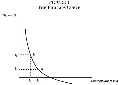
In his 1976 Nobel lecture, “Inflation and Unemployment,” Milton Friedman (1977) traced out three stages in the evolution of the Phillips curve. The first stage featured the simple curve in Figure 1, showing a stable, negative relationship between inflation and unemployment.
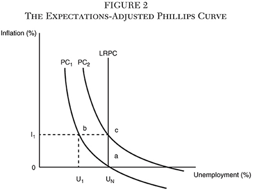
The second stage featured Friedman’s “natural rate hypothesis,” which he first described in his 1967 presidential address to the American Economic Association. In this stage, the short-run Phillips curve is adjusted for expectations and the long-run curve is vertical at the natural rate of unemployment (Friedman 1968). An unexpected increase in inflation initially reduces unemployment. However, once workers and employers fully anticipate higher inflation, they will revise their plans and unemployment will return to its “natural” level consistent with equilibrium real wages and the overall structure of the labor market.2
Figure 2 shows an increase in inflation from 0 percent to I1 temporarily reduces unemployment below its long-run “natural” level UN to U1, say from 4 percent to 3 percent. (No one knows for certain what the actual “natural rate of unemployment” is; it is not observable.) The movement from point a to point b on the initial Phillips curve (PC1) is posited on the assumption that the initial inflation rate is 0 percent. However, once the higher inflation rate is fully recognized by market participants, unemployment will return to UN and PC2 will become the relevant Phillips curve — provided expected inflation remains at I1. Points a and c now lie on the long-run Phillips curve (LRPC), where each point represents a state of full adjustment between actual and expected inflation. Thus, the long-run Phillips curve is vertical. As Meltzer (2009: 287) writes, “The long-run Phillips curve must be vertical because inflation is a nominal variable and unemployment is a real variable. Rational behavior require[s] that any influence of nominal variables on real variables last only as long as it takes markets to learn and adjust.”
The concept of “rational expectations,” first developed by John Muth (1961) and later elaborated upon by Robert Lucas (1987) and Thomas Sargent (1986), provided a strong theoretical case that there could be no tradeoffs between inflation and unemployment — even in the short run. Hence, under the rational expectations framework, systematic monetary policy can have no impact on relative prices, output, or employment. However, if wages and/or prices are sticky and there are costs to acquiring information about job openings, and so on, then activist monetary policies can still have real effects — perhaps for a considerable time (see Humphrey 1986: 126).3
The third stage in the evolution of the Phillips curve is the hypothesis that high and variable inflation plants the seeds for higher future unemployment by distorting relative prices and increasing “regime uncertainty,” thus producing a positively sloped long-run Phillips curve as shown in Figure 3 (adapted from Humphrey 1986: 108).4 As Humphrey explains:
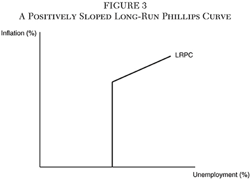
The long-run Phillips curve may become positively sloped in its upper ranges as higher inflation leads to greater inflation variability (volatility, unpredictability) that raises the natural rate of unemployment. Higher and hence more variable and erratic inflation can raise the equilibrium level of unemployment by generating increased uncertainty that inhibits business activity and by introducing noise into market price signals, thus reducing the efficiency of the price system as a coordinating and allocating mechanism [Humphrey 1986: 108].
Milton Friedman considered the possibility of a positively sloped Phillips curve, given the stagflation that occurred in the 1970s. Using inflation lagged one-half year (n 5 0.5), Friedman (1977: 461, Table 1) found that unemployment averaged 6.1 percent from 1971 through 1975 while inflation averaged 6.7 percent. His “tentative hypothesis” was that the positively sloped Phillips curve may be “a transitional phenomenon that will disappear as economic agents adjust not only their expectations but their institutional and political arrangements to a new reality.” He therefore thought that the natural-rate hypothesis would still hold in the very long run, but the “transitional period may well extend over decades” (Friedman 1977: 464–65).
Friedman (1977: 467) recognized that, during the transitional period, “increased volatility of inflation” can distort relative price signals and increase unemployment. Moreover, he believed that, “in practice, the distorting effects of uncertainty, rigidity of voluntary long-term contracts, and the contamination of price signals will almost certainly be reinforced by legal restrictions on price change” (i.e., wage and price controls).
The Great Moderation
During the Great Moderation, roughly from the mid-1980s until 2007, the transition to a more systematic monetary policy that implicitly followed a Taylor-type rule reduced the volatility of inflation and output compared to the stop-go monetary policy that preceded it (see Hakkio 2013). By anchoring inflation expectations and stabilizing the growth of nominal GDP (NGDP) around a trend rate of about 5 percent per year, the Fed improved its credibility and reduced regime uncertainty.
Jerry L. Jordan, former president of the Federal Reserve Bank of Cleveland, described the atmosphere surrounding the Phillips curve during the last two decades of the 20th century:
The macroeconomic developments of the final two decades of the 20th century should have ended any further debate about the notion of some tradeoff between inflation and unemployment. Rates of inflation declined in market economies around the world, regardless of the political systems. Most places also experienced declines in unemployment rates, and where unemployment remained high it was almost universally acknowledged to be the result of national labor market rigidities and regulatory policies. Nowhere was the idea put forth that a bit higher inflation would even temporarily lower the unemployment rates. It seemed — for a while at least — that no minister of finance or central banker would dare to suggest that inflation was too low and that a bit more would in any way be a good thing [Jordan 2012: 22].
Global Financial Crisis and Its Aftermath
The global financial crisis of 2008 ended the Great Moderation and ushered in a new wave of uncertainty associated with unconventional monetary policies. After more than a decade, the inflation rate has remained low despite historically low unemployment, a result that challenges those who continue to place faith in the Phillips curve’s credibility as a forecasting tool to guide monetary policy. As St. Louis Fed President James Bullard (2017) has stated, “the idea that unemployment outcomes are a major factor in driving inflation outcomes in the U.S. economy” cannot be substantiated by the data. “A more important determinant” appears to be “inflation expectations.” He goes on to say:
Despite the empirical evidence suggesting that the Phillips curve relationship is relatively flat, some still argue in favor of raising the U.S. policy rate in an effort to get ahead of the anticipated surge in inflation. Implicit in that argument is the idea that the relationship is nonlinear, meaning the impact on inflation would be much larger once unemployment reached extremely low levels. However, I am not aware of empirical estimates that have made a convincing case for the nonlinear Phillips curve using recent data. For monetary policy purposes, we should not base our notions of what will happen with inflation solely on ideas related to low unemployment.
Even in the face of strong evidence for the flattening of the short-run Phillips curve (i.e., decreases in unemployment have a much smaller impact on inflation than in earlier periods), central banks are reluctant to omit it from their macroeconomic models.5 As Fed Chairman Jerome Powell noted in his April 6, 2018, speech at the Economic Club of Chicago, “Almost all of the participants [at the January 2018 Federal Open Market Committee meeting] thought that the Phillips curve remained a useful basis for understanding inflation.” Yet they recognized “that the link between labor market tightness and changes in inflation has become weaker and more difficult to estimate, reflecting in part the extended period of low and stable inflation in the United States and in other advanced economies” (Powell 2018: 6–7).
The real problem with the Phillips curve is not that it supposes that inflation and unemployment are related, especially in the short run, but that it misconstrues that relation as involving a direct causal influence of unemployment on inflation, and vice versa, when in fact it is changes in aggregate demand that cause changes in both unemployment and inflation. According to Mickey Levy, chief economist at Berenberg:
The Phillips curve, which correctly posits that lower unemployment raises wages, incorrectly presumes that [higher] wages always lead to higher product prices without considering the impact of productivity on production costs, or how nominal aggregate demand influences businesses flexibility to raise product prices. In the 1990s, strong productivity gains were associated with strong gains in real wages, while constraining unit labor costs; that is, the stronger productivity raised the share of nominal GDP that was real. In [the present] expansion, the moderate growth in nominal GDP has constrained wage gains and inflation despite very low unemployment. Not surprisingly, the Phillips curve did not capture either of these dominant trends [Levy 2018].
The Phillips curve is a distraction to the main function of a central bank — namely, to “prevent money itself from being a major source of economic disturbance,” as Milton Friedman observed in his 1968 presidential address (Friedman 1968: 12).
How a Broken Theory Is Still Guiding Policy
At a press conference following the Fed’s Open Market Committee meeting on June 14, 2017, Janet Yellen remarked: “We continue to feel that, with a strong labor market and a labor market that’s continuing to strengthen, the conditions are in place for inflation to move up” (Yellen 2017). Likewise, Fed Chairman Jerome Powell believes the Phillips curve “continues to be meaningful for monetary policy” even though the strength of the relationship between unemployment and inflation “has weakened” (Powell 2018).6
A few years earlier, in 2015, then president of the Federal Reserve Bank of Atlanta, Dennis Lockhart, in an interview with the Wall Street Journal, stated:
I think a policymaker has to act on the view that the basic relationship in the Phillips curve between inflation and [un]employment will assert itself in a reasonable period of time as the economy tightens up, as the resource picture in the economy tightens. I am quite confident that that basic expectation will materialize.… I don’t know if I would quite say that I am resting everything on a model, but I am certainty prepared to get comfortable based on [an] expectation that seems to me to have compelling logic [Hilsenrath 2015, interview with Lockhart].
A final example of how the Phillips curve continues to be treated by Fed officials as a useful guide to policy, even in the face of strong evidence during the last 20 years that the degree of unemployment is a poor indicator of inflation, comes from a working paper prepared by the staff of the Federal Reserve Board’s Divisions of Research & Statistics and Monetary Affairs in 2018:
While inflation appears to be insensitive to labor market slack, policy needs to take proper account of the prospects for persistently tight labor markets leading to higher inflation, or other imbalances, that could eventually endanger prospects on the employment side of [the Fed’s] policy mandate [Erceg et al. 2018: 18].
All of the forgoing examples show that central bankers are not yet willing to discard the Phillips curve as a policy tool, even though the evidence for a downward sloping curve is meager. Indeed, as early as 2002, William Niskanen, a former member of President Ronald Reagan’s Council of Economic Advisers, declared: “The concept of a Phillips curve should be considered empty when most of the variation in the data must be explained by shifts in this presumed relation. In any case, the Phillips curve proved to be a poor basis for forecasting and a worse guide to policy” (Niskanen 2002: 194).
Using annual data from 1960 through 2001, Niskanen found that “there is no tradeoff of unemployment and inflation except in the same year,” and that “in the long term, the unemployment rate is a positive function of the inflation rate” (Niskanen 2002: 198). During the 1970s, inflation and unemployment both increased, as the United States experienced stagflation, and since 2009, unemployment has turned sharply lower while inflation has remained low.
Nevertheless, the existence of even a transient and loose relation between inflation and unemployment provides policymakers with the illusory hope that they can exploit that relation to achieve desired policy goals. The idea that a little more inflation is desirable in return for a little less unemployment is appealing to both policymakers and politicians, both of whom are inclined to overemphasize the short run and discount the long run. That is why economic fallacies have a tendency to reappear, especially when politicians can win votes by resurrecting them. Protectionist rhetoric is one common example; the idea that a little inflation is a good thing is another.
Although the Phillips curve has been discredited, it is not really dead and so distracts from alternative ideas for conducting monetary policy that offer a better chance of achieving long-run price stability and promoting economic stability and growth. The still-lingering influence of circa. 1965 Keynesianism — with its emphasis on short-run remedies for long-run problems, its distrust of the market adjustment process, and its dismissal of the quantity theory of money — downplays the point, clearly recognized by F. A Hayek in 1960, that “the stimulating effect of inflation will … operate only so long as it has not been foreseen; as soon as it comes to be foreseen, only its continuation at an increased rate will maintain the same degree of prosperity” (Hayek 1960: 331). Hayek went on to criticize the myopic view of policymakers:
The inflationary bias of our day is largely the result of the prevalence of the short-term view, which in turn stems from the great difficulty of recognizing the more remote consequences of current measures, and from the inevitable preoccupation of practical men, and particularly politicians, with the immediate problems and the achievement of near goals [Hayek 1960: 333].
The Phillips curve gives policymakers a justification to try to fine-tune the economy, but it is a weak reed on which to base policy — and it fails to recognize the limits of monetary policy.7
A Better Framework for Monetary Policy
Instead of relying on a flawed Phillips curve analysis to guide policy, Fed officials should focus on the underlying causes of both undesired changes in inflation and cyclical fluctuations in unemployment. In turn, the Fed’s dual mandate to achieve maximum employment and price stability, which is flawed by assuming a tradeoff between inflation and unemployment, should be replaced by a single target, preferably keeping NGDP on a level growth path.8 Doing so would increase the credibility of monetary policy, reduce regime uncertainty, mitigate business fluctuations, and avoid stop-go monetary policy. Niskanen (2008: 377) argued that “the intent of Congress would be better served and monetary policy would be more effective if Congress instructed the Federal Reserve to establish a monetary policy that reflects both their concerns in a single target.” He did so because he clearly recognized the failure of forecasting inflation under a Phillips curve framework and, hence, the merits of a nominal income target over an inflation target (with the unemployment rate serving as a poor proxy for likely inflation).9
One benefit of a rule designed to keep nominal income on a steady growth path is that it bypasses the issue of assigning weights under the Fed’s dual mandate to achieve price level stability and maximum employment. All that needs to be done is to set a target path for the growth of nominal spending (i.e., the sum of real output growth and inflation). Market forces will then determine real growth.
Peter Ireland nicely summarizes the benefits of NGDP targeting over a problematic reliance on the Phillips curve as a guide to monetary policy:
As the sum of real GDP growth and nominal price inflation, NGDP growth conveniently captures, in a single number, the Fed’s performance in satisfying both sides of its dual mandate for maximum sustainable growth with stable prices. At the same time, however, NGDP, precisely because it is a nominal variable, measured in units of dollars, is under the central bank’s control in the long run.… Moreover, the Fed’s ability to regulate the growth rate of NGDP does not depend on the stability of the Phillips curve.… [I]n the current environment, where various nonmonetary forces may well be causing the very low rate of measured unemployment to overstate the true degree of resource utilization in the U.S. economy, focusing instead on the real component of NGDP growth guards against one of the risks alluded to in Powell’s remarks: a policy stance that becomes inappropriately restrictive out of concern for inflationary pressures working through a misperceived Phillips curve.
Finally, as noted by Tobin (1983) and McCallum (1985), the equation of exchange MV5PY identifies nominal income (PY) as a measure of the money supply (M) that gets adjusted automatically for shifts in velocity (V). Thus, analyses based on the behavior of NGDP growth provide a monetarist cross-check against mainstream Keynesian approaches, like Powell’s, organized around the Phillips curve instead. According to this monetarist view, interactions between trends in M, reflecting monetary policy actions that affect the money supply, and V, interpreted following Friedman (1956) with reference to the determinants of money demand, replace those between the actual and natural rates of unemployment as the key mechanisms determining inflation [Ireland 2019a: 52–53].
Congress should put the Phillips curve to bed and consider the case for a nominal GDP (or domestic final sales) target. One step toward that goal would be to add nominal GDP growth to the Fed’s Summary of Economic Projections, a proposal first made by Jeffrey Frankel (2019: 461–70).
Conclusion
Instead of continuing to hold onto the discredited presumption of a tradeoff between inflation and unemployment, policymakers should focus on the misallocative and distributive effects of activist monetary policy. The Fed needs to recognize that the Phillips curve is not a reliable policy compass. A monetary policy based on short-run activism, such as that implied by a “data-dependent” Fed, is not a good substitute for one based on a transparent, long-run strategy guided by a robust monetary rule. Policymakers should heed the advice of Hayek, who in 1975 wrote:
What we must now be clear about is that our aim must be, not the maximum of employment that can be achieved in the short run, but a “high and stable level of employment.” We can achieve this, however, only through the reestablishment of a properly functioning market which, by the free play of prices and wages, establishes the correspondence of supply and demand for each sector.
Though monetary policy must prevent wide fluctuations in the quantity of money or in the volume of the income stream, the effect on employment must not be its dominating consideration. The primary aim must again become the stability of the value of money. The currency authorities must again be effectively protected against the political pressure that today forces them so often to take measures that are politically advantageous in the short run but harmful to the community in the long run [Hayek (1975) 1979: 17].
It has been more than 40 years since Hayek made those recommendations for changes in the framework for monetary policy, yet we are still in search of a monetary constitution.10
The Phillips curve has diverted attention from the search for a monetary constitution and a rules-based regime by promoting the idea that central banks can use expansionary monetary policy to lower unemployment — and, hence, that discretionary policy is to be preferred to a rules-based regime. Macroeconomic models used by the world’s central banks still rely on the Phillips curve as a tool for their inflation forecasts, even though those forecasts have been unreliable.
Today, the United States has historically low unemployment while inflation has stayed at less than 2 percent for more than a decade. Those facts alone should convince policymakers that the Phillips curve is a poor guide for monetary policy.
References
Beckworth, D. (2017) “The Knowledge Problem in Monetary Policy: The Case for Nominal GDP Targeting.” Mercatus on Policy Series (July 18). Mercatus Center, George Mason University.
Bullard, J. (2017) “Does Low Unemployment Signal a Meaningful Rise in Inflation?” Federal Reserve Bank of St. Louis Regional Economist (Third Quarter).
Dorn, J. A. (1987) “The Search for Stable Money: A Historical Perspective.” In J. A. Dorn and Anna J. Schwartz (eds.), The Search for Stable Money: Essays on Monetary Reform, 1–28. Chicago: University of Chicago Press.
_________ (2001) “The Limits of Monetary Policy.” Cato Handbook for Congress, 108th Congress, 247–56. Washington: Cato Institute.
_________ (2018) “Monetary Policy in an Uncertain World: The Case for Rules.” Cato Journal 38 (1): 81–108.
_________ (2019) “Myopic Monetary Policy and Presidential Power: Why Rules Matter.” Cato Journal 39 (3): 577–95.
Erceg, C.; Hebden, J.; Kiley, M.; López-Salido, D.; and Tetlow, R. (2018) “Some Implications of Uncertainty and Misperception for Monetary Policy.” Finance and Economics Discussion Series 2018-059. Washington: Board of Governors of the Federal Reserve System.
Frankel, J. (2019) “Should the Fed Be Constrained?” Cato Journal 39 (2): 461–70.
Friedman, M. (1956) “The Quantity Theory of Money: A Restatement.” In Studies in the Quantity Theory of Money, 3–21. Chicago: University of Chicago Press.
_________ (1968) “The Role of Monetary Policy.” American Economic Review 58 (1): 1–17.
_________ (1977) “Nobel Lecture: Inflation and Unemployment.” Journal of Political Economy 85 (3): 451–72.
Gordon, R. J. (1985) “The Conduct of Domestic Monetary Policy.” In A. Ando et al. (eds.), Monetary Policy in Our Times. Cambridge, Mass.: MIT Press.
Hakkio, C. S. (2013) “The Great Moderation.” Federal Reserve History blog (November 22): www.federalreservehistory.org/essays/great_moderation.
Hall, T. E., and Hart, W. R. (2012) “The Samuelson–Solow Phillips Curve and the Great Inflation.” History of Economics Review 55 (Winter): 62–72.
Hayek, F. A. (1960) The Constitution of Liberty. Chicago: University of Chicago Press.
_________ ([1975] 1979) Unemployment and Monetary Policy: Government as Generator of the Business Cycle. San Francisco: Cato Institute. Revised edition of Full Employment at Any Price? London: Institute of Economic Affairs (1975).
Higgs, R. (1997) “Regime Uncertainty: Why the Great Depression Lasted So Long and Why Prosperity Resumed after the War.” The Independent Review 1 (4): 561–90.
Hilsenrath, J. (2015) “Excerpts from Atlanta Fed’s Lockhart Interview.” Wall Street Journal (August 4).
Humphrey, T. M. (1986) Essays on Inflation, 5th ed. Richmond, Va.: Federal Reserve Bank of Richmond.
Ireland, P. N. (2019a) “Economic Conditions and Policy Strategies: A Monetarist View.” Cato Journal 39 (1): 51–63.
_________ (2019b) “Independence and Accountability via Inflation Targeting: Strengthening the Foundations for Successful Monetary Policymaking.” Paper presented at the Cato Institute’s 37th Annual Monetary Conference, Washington, D.C., November 14.
Jordan, J. L. (2012) “Friedman and the Phillips Curve.” In Sound Money: Why It Matters, How to Have It, 9–29. Ottawa, Ontario: Macdonald-Laurier Institute.
Levy, M. D. (2018) “U.S. Nominal GDP Acceleration: Pay More Attention to It.” Economics Macro News, Berenberg Capital Markets (August 6).
Lipsey, R. G. (1960) “The Relation between Unemployment and the Rate of Change in Money Wages in the United Kingdom, 1862–1957: A Further Analysis.” Economica 27 (105): 1–31.
Lucas, R. E. Jr. (1987) Models of Business Cycles. Oxford: Basil Blackwell.
McCallum, B. T. (1985) “On Consequences and Criticisms of Monetary Targeting.” Journal of Money, Credit, and Banking 17 (November, Part 2): 570–97.
_________ (1989) Monetary Economics: Theory and Policy. New York: Macmillan.
Meltzer, A. H. (1989) “On Monetary Stability and Monetary Reform.” In J. A. Dorn and W. A. Niskanen (eds.) Dollars, Deficits, and Trade, 63–85. Boston: Kluwer.
_________ (2009) A History of the Federal Reserve: Volume 2, Book 1, 1951–1969. Chicago: University of Chicago Press.
Muth, J. A. (1961) “Rational Expectations and the Theory of Price Movements.” Econometrica 29 (6): 315–35.
Ng, M.; Wessel, D.; and Sheiner, L. (2018) “The Hutchins Center Explains: The Phillips Curve.” Brookings Up Front (August 21). Available at www.brookings.edu/blog/up-front/2018/08/21/the-hutchins-center-explains-the-phillips-curve.
Niskanen, W. A. (1992) “Political Guidance on Monetary Policy.” Cato Journal 12 (1): 281–86.
_________ (2002) “On the Death of the Phillips Curve.” Cato Journal 22 (2): 193–98.
_________ (2008) “Monetary Policy and Financial Regulation.” Cato Handbook for Policymakers, 7th ed., 377–84. Washington: Cato Institute,
Phelps, E. S. (1967) “Phillips Curves, Expectations of Inflation, and Optimal Unemployment over Time.” Economica 34 (135): 254–81.
_________ (1968) “Money-Wage Dynamics and Labor-Market Equilibrium.” Journal of Political Economy 76 (July-August): 678–711.
Phillips, A. W. (1958) “The Relation between Unemployment and the Rate of Change of Money Wages in the United Kingdom, 1861–1957.” Economica 25 (100): 283–99.
Plosser, C. I. (2014) “A Limited Central Bank.” Cato Journal 34 (2): 201–11.
Powell, J. H. (2018) “The Outlook for the U.S. Economy.” Speech given at the Economics Club of Chicago (April 6).
Samuelson, P. A., and Solow, R. M. (1960) “Analytical Aspects of Anti-Inflation Policy.” American Economic Review (Papers and Proceedings) 50 (2): 177–94.
Sargent, T. J. (1986) Rational Expectations and Inflation. New York: Harper & Row.
Selgin, G. (2017) “Bill Niskanen: Monetary Policy Radical.” Alt‑M (December 21).
Selgin, G.; Beckworth, D.; and Bahadir, B. (2015) “The Productivity Gap: Monetary Policy, the Subprime Boom, and the Post-2001 Productivity Surge.” Journal of Policy Modeling 37 (2): 189–207.
Steelman, A. (2011) “The Federal Reserve’s ‘Dual Mandate’: The Evolution of an Idea.” Federal Reserve Bank of Richmond Economic Brief (December).
Stock, J. H., and Watson, M. W. (2019) “Slack and Cyclically Sensitive Inflation.” NBER Working Paper No. 25987 (June).
Sumner, S. B. (2014) “Nominal GDP Targeting: A Simple Rule to Improve Fed Performance.” Cato Journal 34 (2): 315–37.
Tobin, J. (1983) “Monetary Policy: Rules, Targets, and Shocks.” Journal of Money, Credit, and Banking 15 (November): 506–18.
Volcker, P. (1981) Federal Reserve’s First Monetary Policy Report for 1981. Hearings before the U.S. Senate Committee on Banking, Housing, and Urban Affairs (February 25 and March 4). Washington: U.S. Government Printing Office.
White, L. H.; Vanberg, V. J.; and Köhler, E. A. (eds.) (2015) Renewing the Search for a Monetary Constitution. Washington: Cato Institute.
Yeager, L. B. (ed.) (1962) In Search of a Monetary Constitution. Cambridge, Mass.: Harvard University Press.
Yellen, J. (2017) “Transcript of Chair Yellen’s Press Conference” (June 14). Available at www.federalreserve.gov/mediacenter/files/FOMCpresconf20170614.pdf.
1 In an endnote, the authors suggest: “The diagrams for the sub-periods in Phillips’s paper might also have alerted Samuelson and Solow to the fact that the Phillips curve relation only seemed to be stable under fixed exchange rates which helped to anchor inflation expectations” (Hall and Hart 2012: 69, n.7).
2 For a more detailed description of the adjustment process from an unanticipated increase in nominal aggregate demand, see Friedman (1968: 100–11; 1977: 456–57). Friedman gives credit to Edmund S. Phelps for his groundbreaking work in developing the natural rate hypothesis, for which he received the Nobel Memorial Prize in Economic Sciences in 2016 (see Phelps 1967, 1968).
3 Friedman (1968: 11) estimated “that the initial effects of a higher and unanticipated rate of inflation last for something like two to five years; that this initial effect then begins to be reversed; and that a full adjustment to the new rate of inflation takes … a couple of decades.” The adjustment process would be faster, he said, in countries experiencing “more sizable changes” in the rate of inflation.
4 Robert Higgs (1997) coined the term “regime uncertainty,” which he used to refer to the uncertainty caused by fiscal and regulatory policies that attenuated private property rights by decreasing expected returns on capital. In the case of a discretionary government fiat money regime, moving to a monetary rule would help reduce uncertainty about the future value of money and improve the climate for making private investment decisions (Dorn 2018, 2019).
5 Stock and Watson (2019: 1) find that the slope of the Phillips curve (measured by the change in inflation relative to the change in the unemployment gap), has gone from 20.48 in 1960–83 to 20.26 in 1984–99, and to 20.03 in 2000–2019Q1, which is not statistically different from zero.
6 By “weakened,” Powell means the slope of the Phillips curve has flattened: large decreases in unemployment have not had much impact on inflation. The rate of unemployment has gone from 10 percent in October 2009 to less than 4 percent today, while inflation has remained relatively low at less than 2 percent per year.
7 On the limits of monetary policy, see Friedman (1968), Plosser (2014), and Dorn (2001).
8 On the case for an NGDP target, see Sumner (2014); Selgin, Beckworth, and Bahadir (2015); and Beckworth (2017). Earlier proponents include Gordon (1985), McCallum (1989: chap. 16), and Meltzer 1989). Niskanen (1992: 284) favors targeting nominal domestic final sales (NDFS) and argues that keeping nominal demand on a stable growth path is superior to a “price rule” and a “money rule.” Unlike a price rule (e.g., inflation targeting), “a demand rule.… does not lead to adverse monetary policy in response to unexpected … changes in supply conditions.” Even more important, a demand rule, unlike a money rule, “accommodates unexpected changes in the demand for money” (i.e., in the velocity of money). See also Frankel (2019: 464–65).
9 On Niskanen’s ideas for reforming the monetary framework, see Selgin (2017).
10 On the search for a monetary constitution and stable money, see Yeager (1962); Dorn (1987); and White, Vanberg, and Köhler (2015).
About the Author


This work is licensed under a Creative Commons Attribution-NonCommercial-ShareAlike 4.0 International License.