The most recent Census (2018a) report does show more encouraging trends, with real median household income rising 5.2 percent in 2015, 3.1 percent in 2016, and 1.8 percent in 2017 (p. 27). But this recovery was from a low level in 2014, and the Census estimate for 2017 is still only 2.2 percent above the level in 1999, implying near-stagnation (at growth of only 0.12 percent per year) over nearly two lost decades.² After correction for a better deflator and for household size, and considering trend rather than specific endpoints, the outcome over this period is far better.

Calculating Trend Income Growth

A classic problem in calculating long-period growth rates is the risk of arriving at misleading conclusions if the rate is calculated simply between two endpoints. If the particular endpoint years chosen show unusually low income in the initial year and unusually high income in the ending year, the result will be to exaggerate the long-term growth rate (and vice versa if the opposites are true). For this reason, it is a classic practice to estimate long-term growth rates using regressions of the logarithm of income on time, in effect giving every year in the time span an equal weight rather than being dependent on just the beginning year and the final year.

If income grows at a constant annual rate of g, income in year t is Y_t, and Y₀ what the trendline indicates would have been expected as the base income in the year prior to the beginning of the series, then:

where “e” is the base of the natural logarithm.³ Taking the logarithm of both sides yields:

A statistical regression of the logarithm of income against time will thus yield a constant term that is the logarithm of the trendline starting point value and a linear coefficient on time that equals the growth rate “g”.

Because even a casual inspection of the data does show a clear slowdown in the pace of income growth after 2000, however, it is important to incorporate a shift variable that allows the measured growth rate to decline. One can think of the level of income in the period after 2000 as being the product of the level that would have been predicted using the trend growth rate through 2000, multiplied by a factor that captures the shift in the growth rate after 2000. Thus,

where T 5 0 for all years before 2000 and then takes the value of 1 for 2000, 2 for 2001, and reaches 17 for 2016.⁴ The corresponding logarithmic form is then

Whereas the trendline growth rate will then be simply g in the period before 2000, thereafter the trend growth rate will be g + δ. In the logarithmic form, the annual growth rate equals the change in the logarithm divided by the number of years for the period in question. Both t and T rise by unity for each successive year after 2000, so the annual growth rate in the period after 2000 is g + δ. The expectation is that in the statistical estimate, d will be found to be negative. A key question is whether the absolute value of d is greater than g, in which case the trendline turns negative after 2000, or less than g, so that growth continues to be positive but at a lower rate than before.

Choosing the Right Deflator

In its annual report on incomes and poverty, Census (2018a) reports real median household income over time deflating by a “research” version of the consumer price index (CPI-U-RS, or CPI_RS), compiled by the Bureau of Labor Statistics. In contrast, in its corresponding analysis, the Congressional Budget Office (CBO, 2016, 2018) deflates using the personal consumption expenditure (PCE) from national accounts, prepared by the Bureau of Economic Analysis. Over the past five decades, the cumulative rise in the CPI_RS is substantially greater than that in the PCE. Thus, with the average for 1967–70 as an index base of 100, by 2017 prices rose to an index of 603.7 in the CPI_RS but only 540.2 in the PCE.⁵ Cumulative inflation over this period was thus about 12 percent higher in the CPI_RS than in the PCE. Most analysts consider the PCE to be the better index because it takes much better account of substitutability as relative product prices change.⁶

Adjustment for Household Size

Average household size declined from 3.28 persons in 1967 to 2.62 by 2000 and 2.54 by 2017 (Census 2017b). Larger households can be expected to have greater income earning potential from the availability of more potential workers. It is thus important to adjust for household size in assessing the long-term growth of household income. Otherwise, the larger households at the beginning of the period would tend to exaggerate the income levels relative to household incomes toward the end of the period. However, the economic significance of size is likely to be less than linear. From the earning standpoint, the additional household members in the early period would tend to have included the young and the elderly, so income potential would not have been expected to be higher by the full proportion of larger household size. From the consumption standpoint, economies of scale in sharing housing costs (for example) would similarly imply that the economically meaningful size rises by less than the number of residents.

The CBO (2016, 2018) uses the square root as the metric for standardizing household size in assessing income trends. Thus, normalizing for family size would involve dividing 1967 median household income by the square root of 3.28 and comparing it to median household income in 2016 divided by the square root of 2.54. This normalization would shrink the 1967 base by 12.2 percent to make it comparable to the 2017 endpoint.⁷ In contrast, shrinkage linearly with respect to size would cut reported household income at the beginning of the period by 22.6 percent to make it comparable to income at the end of the period.⁸ The estimates that follow adopt the CBO’s convention of normalizing by the square root of size.

The Census also reports incomes by families, defined as a group of two or more people residing together and related by birth, marriage, or adoption. However, single-person households are excluded from this group by definition. As families defined in this way accounted for only 80.1 percent of the population in 2017, whereas households represented 99.7 percent, most analyses focus on the household rather than family data.⁹

Long-Term Trends

Figure 1 shows the path of median household income in real 2017 dollars for three alternative measures. The top line reports the Census estimates, which use the CPI-U-RS as the deflator. The intermediate line shows the same data after replacing the CPI-U-RS with the PCE as deflator. The bottom line shows the PCE-deflated series after a further adjustment to normalize for household size (by square root). All three lines converge for 2017, at a median household income of $61,372.

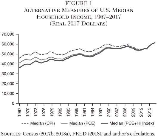
Because the PCE-deflated series and especially the size-normalized series start out lower than the unadjusted series reported by the Census, they show steeper lines. The average annual growth rate over the full period will thus be higher for the PCE-deflated series than the CPI-U-RS series, and growth will be even higher for the series that not only deflates using the PCE but also adjusts for household size. All three series show a decline from 2007 to 2011, followed by a rebound by 2016. However, the Census version shows stagnation after a high point at 2000, whereas the other two series show higher levels by 2007 than in 2000.

Table 1 reports the results of applying the log-linear regression estimates of growth rates using equation (4) discussed earlier. The t-statistics shown in parentheses all indicate significance at the 5 percent level or better,¹⁰ and the adjusted R² reaches 94 percent in the estimates with PCE as the deflator and adjusting for household size.

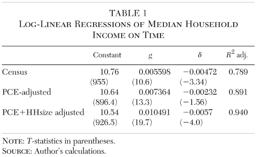
The column for “g” indicates that whereas the Census estimates showed annual growth of only 0.56 percent from 1967 through 1999, replacing the CPI-U-RS deflator by the PCE boosts this rate to 0.74 percent, and adjusting the PCE-deflated series for household size boosts this period’s growth rate further to 1.05 percent. The column for “δ” indicates that this long-term annual growth rate shifts downward by about 0.47 percent after 1999 for the Census series, 0.2 percent for the PCE-deflated series, and by 0.57 percent for the series additionally adjusting for household size. As a consequence, for 2000–17 the trendline growth (g − δ) falls to less than one-tenth of 1 percent annually in the Census series, but remains considerably more substantial at 0.5 percent annually in the PCE-deflated series and 0.48 percent annually in the series additionally adjusted for household size.

Trendline versus the 1999/2014 Comparison

Returning to Figure 1, it is clear why some presidential candidates in early 2016 were able to say that median household incomes in the latest year available, 2014, were well below their level in 1999, using the data as reported by the Census. Even after adjustment to the PCE and for household size, the level in 2014 was slightly below that in 1999.¹¹

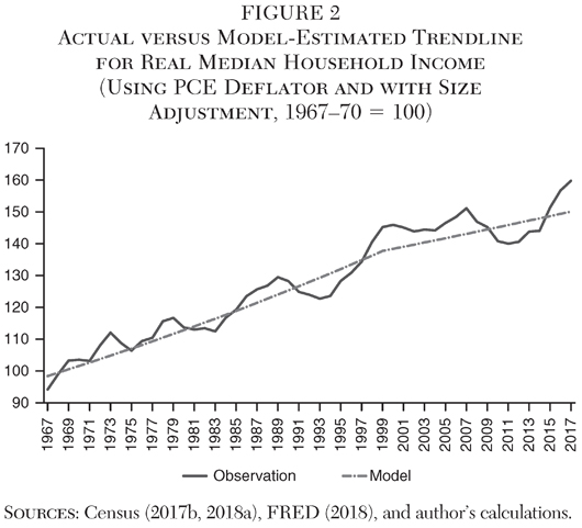
Figure 2 uses the final model shown in Table 1 to provide the trendline estimate of income, after converting to an index with 1967–70 = 100. However, as shown in Figure 2, even using the estimates adjusted for PCE and household size, the real income levels in 1999 and 2000 were well above trendline. This gap is not surprising considering that real growth had been unusually high in the late 1990s, the era of the dot-com bubble. In contrast, the 2014 level was well below even the new slower-paced trendline, reflecting the long shadow of the Great Recession. If growth from 1999 to 2014 is judged solely by these two endpoints, the annual average was − 0.5 percent in the Census estimates, but virtually zero in the adjusted estimates.¹² However, using the model in the final section of Table 2, trendline growth in this period was 0.48 percent annually for the adjusted series. This comparison emphasizes the importance of examining the overall trendline rather than choosing specific endpoint years for a comparison. Moreover, with the observations exceeding the model of equation (4) by 2015–17, there would seem to be reasonable chances that inclusion of the 2018 outcome would reduce the size of the post-1999 growth-subtraction parameter “δ.”

Trendline Real Median Household Income by 2017

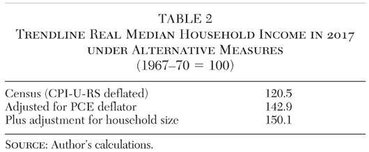
The alternative trendline log-linear estimates of Table 2 can be used to identify how much real median household income has risen under alternative measures. These equations are converted from logarithmic to arithmetic levels (taking the exponential) and converted to an index of 1967–70 = 100. Table 2 shows the resulting index levels for 2017 for these three equations.

The estimates in Table 2 indicate that after correction using a better deflator, and after normalization for household size, over the past 50 years trendline real median household income has risen by 50 percent rather than by just 21 percent as calculated using the most widely cited Census results.¹³

Lower-Middle Incomes

An important narrative in the U.S. political economy has been that the lower the household is in the income distribution, the more it will have lagged behind national average income growth.¹⁴ It is thus useful to examine whether incomes have grown more slowly for lower-middle income households than for median household income. The Census (2018b) estimates provide information on average household incomes by quintile of the income distribution. As a measure of “lower-middle” incomes, it is useful to examine the mean income in the second quintile (20–40 percent). The third quintile (40–60 percent) essentially represents the median of all households, already considered above.¹⁵

When the same adjustments are applied to the mean household incomes for the second quintile as applied in the analysis above for the overall median income (conversion to PCE deflator and adjustment for household size), and once again using 1967–70 as an index base of 100, the resulting path for real lower-middle incomes is that shown in Figure 3. The figure also shows the corresponding measure of median household income (the same as shown by the individual year observations in Figure 2).

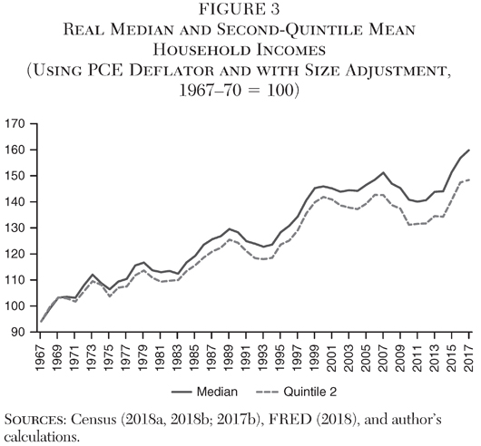
Growth in the mean income of the second quintile does lag behind that of the median for all households, although not by a particularly large amount. From 1967–70 to 2014–17, the ratio of the second quintile mean to the overall median fell from 0.621 to 0.579, indicating that average annual growth was 0.15 percent lower for the second quintile than for the median.

On the basis of this comparison, the implication is that real household incomes have not been stagnant over the past 50 years even for the second quintile. Whereas the total trendline increase over this period for the median household was 50.1 percent as shown in Table 2, the corresponding increase would have been about 40 percent for the second quintile (Figure 3).¹⁶

Influence of Racial Composition

White households have higher median incomes than those of the rest of the population. Over the past five decades the number of white households has risen more slowly than the number of all other households. As a consequence, when assessing the growth performance of household incomes, there can be said to be a downward bias derived from changing racial composition.

There has been considerable narrowing in the racial income differential over the past five decades. In 1972, non-Hispanic white households had a median income that was 1.67 times as high as the median income of all other households; by 2017, this ratio had fallen to 1.42.¹⁷ Other things being equal, if racial composition had remained unchanged, the median income of all households by 2017 would have been 6.1 percent higher than the level actually observed.¹⁸

The Census (2018c) data do not provide detail on household size by race prior to 1999. From 1999 to 2017, average household size declined from 2.60 persons to 2.53 for the population as a whole.¹⁹ For non-Hispanic whites, the change over this period was from 2.43 persons to 2.37; for all others, the change was from 3.10 persons to 2.85. The log-linear time trend of PCE-deflated, size-adjusted household income in this period was an annual increase of 0.37 percent for white non-Hispanic households, and 0.62 percent for all others.²⁰ The ratio of “other” to non-Hispanic white median size-adjusted household income rose from 0.61 in 1999 to 0.64 in 2017.

Census versus Congressional Budget Office

Estimates of trends in median household income by the Congressional Budget Office (CBO 2018) support the findings here that the Census (2018a) estimates tend to understate growth in real median household income. The CBO uses the PCE as the deflator, as is done here. It also uses the square root of the number of household members to normalize for household size when assigning a household to a percentile in the income distribution.

The CBO reports trends for income before taxes and transfers, as well as income after taxes and transfers. Even the before-transfers concept includes “social insurance benefits,” including Social Security benefits, Medicare benefits, unemployment insurance, and workers compensation (CBO 2018: 37). Because Medicare benefits are estimated based on average cost to the government of providing the benefits, this category of income would be excluded from the Census data on money income (which excludes imputed benefits not received in money). The CBO income data also include as income to the worker the payments by employers for health insurance premiums; the employer’s share of Social Security, Medicare, and federal unemployment insurance payroll taxes; and, somewhat surprisingly, “the share of corporate income taxes borne by workers,” as the concept is before taxes and transfers. None of these categories would be included in the Census measure, money income. Especially in view of the rising cost of health insurance and Medicare benefits and taxes, one would expect the CBO measure to show a greater increase in income before taxes and transfers than found by Census, even after adjusting the Census estimates for deflating by the PCE and adjusting for family size.

The CBO (2018: 4) estimates that before taxes and transfers, household income of the middle three quintiles rose by 28 percent from 1979 to 2014. In the adjusted Census estimates shown for the median in Figure 3, the rise from 1979 to 2014 was somewhat lower at 24 percent, reflecting the narrower money income concept. For the concept of income after taxes and transfers, the CBO estimates show an even more favorable trend, with an increase of 42 percent from 1979 to 2014 for the middle three quintiles.

The CBO estimates seem to have received little attention in the public debate on whether household incomes have stagnated. Thus, a search for “median income” plus “Census Bureau” in the month after the release of the 2017 Census report (Census 2017a) yielded 61 articles in the leading financial press, whereas a corresponding search for “median income” plus “Congressional Budget Office” found no press mention at all in the month following publication of its 2016 report (CBO 2016).²¹ One likely reason for the lower public profile of the CBO estimates is that they are typically reported with a lag of three to four years, whereas those of the Census are reported with a lag of one year.²² The longer lag in part reflects the CBO’s use of Statistics of Income (SOI) compiled by the Internal Revenue Service, rather than just the Current Population Survey (CPS) data of the Census (although the CBO uses the CPS to map supplementary data to the households in the SOI survey).

Conclusion

A popular political narrative is that middle- and lower-middle incomes in the United States have fallen since 1999 and have been stagnant for decades. However, when the most widely cited (Census 2018a) data are adjusted using a better price deflator, changes in household size are taken into account, and long-term trendlines are used for the comparison rather than picking endpoints using the unusually high base years of 1999 or 2000, it is found that household incomes have continued to grow, albeit at a slower pace. The trendline shows annual real growth of 1.0 percent for 1967–99 and 0.48 percent for 2000–17. For the whole period second-quintile incomes have lagged growth of median incomes, but only modestly (by 0.15 percent per year). From their averages in 1967–70, trendline real median household incomes by 2017 had risen 50.1 percent, and second-quintile incomes rose about 40 percent.

The overall implication is that it is a mistake to judge that American capitalism is broken because the middle- and lower-middle classes have seen no gains for decades. Moreover, the slowdown after 2000 included the period of the Great Recession, the most extreme shock to the economy since the 1930s. Some return to higher growth than the 2000–17 trend of 0.48 percent can be expected as the Great Recession recedes further into the past and the relative weight of more normal years increases.

References

BLS (Bureau of Labor Statistics) (2011) “Differences between the Consumer Price Index and the Personal Consumption Expenditures Price Index.” Focus on Prices and Spending 2 (3): 1–7.

__________ (2018) CPI-All Urban Consumers (Current Series). Washington: BLS (April).

CBO (Congressional Budget Office) (2016) The Distribution of Household Income and Federal Taxes, 2013. Washington: CBO (June).

__________ (2018) The Distribution of Household Income and Federal Taxes, 2014. Washington: CBO (March).

Census (U.S. Census Bureau) (2014) “Income and Poverty in the United States: 2013.” Current Population Reports (September).

__________ (2015) “Income and Poverty in the United States: 2014.” Current Population Reports (September).

__________ (2017a) “Income and Poverty in the United States: 2016.” Current Population Reports (September).

__________ (2017b) Historical Households Tables. Table HH-4. Available at www.census.gov/data/tables/time-series/demo/families/households.html.

__________ (2018a) “Income and Poverty in the United States: 2017.” Current Population Reports (September).

__________ (2018b) Historical Income Tables: Households. Table H-3. Available at www.census.gov/data/tables/time-series/demo/income-poverty/historical-income-households.html.

__________ (2018c) “Size of Household by Median and Mean Income.” Table H-11. Available at www.census.gov/data/tables/time-series/demo/income-poverty/historical-income-households.html.

__________ (2018d) “Selected Characteristics of Families by Total Money Income in 2017.” Data: FINC-01. Available at www.census.gov/data/tables/time-series/demo/income-poverty/cps-finc/finc-01.html.

__________ (2018e) QuickFacts United States. Available at www.census.gov/quickfacts/fact/table/US/PST045216.

FRED (Federal Reserve Bank of St. Louis) (2018) “Personal Consumption Expenditures: Chain-type Price Index.” Available at https://fred.stlouisfed.org/series/PCEPI.

Furth, S. (2017) “Measuring Inflation Accurately.” Backgrounder No. 3213. Washington: Heritage Foundation.

Irwin, N. (2016) “The Economic Expansion Is Helping the Middle Class, Finally.” New York Times (September 13).

Leonhardt, D. (2017) “Our Broken Economy, in One Simple Chart.” New York Times (August 7).

Missouri Census Data Center (2018) Measures of Income in the Census. Jefferson City, Mo.

Sacerdote, B. (2017) “Fifty Years of Growth in American Consumption, Income, and Wages.” NBER Working Paper No. 23292 (March).

Winship, S. (2015) “Debunking Disagreement Over Cost-Of-Living Adjustment.” Forbes (June 15).

¹Thus, in the campaign, candidate Donald Trump stated, “Household incomes are down more than $4,000 since the year 2000”; and candidate Bernie Sanders stated, “Since 1999, the typical middle-class family has seen its income go down by almost $5,000 after adjusting for inflation.” See www.politifact.com/truth-o-meter/statements/2016/jul/21/donald-trump/donald-trump-largely-right-household-incomes-are-d; www.politifact.com/truth-o-meter/article/2015/jul/24/closer-look-old-bernie-sanders-talking-point. Both statements were broadly correct given the data in Census (2014, 2015), although technically the number cited by Mr. Sanders referred to household income, not family income.

²That is: ln (1.022)/18 = 0.0012.

³The absolute change in income from a unit increase in the number of years “t” is the derivative of the right-hand side, or dY/dt = gY₀e^gt. Dividing both sides by Y₀e^gt gives the proportionate change, or growth rate, namely “g.”

⁴Because T has the value 0 prior to 2000, the final term following the multiplication sign in equation (3) becomes unity for all years before 2000, leaving the equation unchanged from equation (1) for those years.

⁵Calculated from Census (2018a: 26) for the CPI_RS and FRED (2018) for the PCE.

⁶The PCE applies a Fisher-ideal chain-type index, which is the geometric mean of the Laspeyres index using base period weights and the Paasche index using end period weights. The CPI_RS only allows for substitutability in this fashion at an extremely detailed level (each of 8,018 goods and services categories) and applies a Laspeyres index for their aggregation. For a detailed analysis, see Furth (2017). Winship (2015) also emphasizes this difference. There are also differences in category weights and in scope. One area in which the PCE tends to show higher inflation is in health care, as it includes prices for government- or employer-provided health care rather than just out-of-pocket consumer expenses in the CPI (BLS 2011). Based on various estimates, Furth (2017) argues that even the PCE overstates inflation by about 0.4 percent per year because of inadequate measurement of quality improvement.

⁷That is: √2.54 = 1.59; √3.28 = 1.81; 1.59/1.81 = 0.878.

⁸That is: 2.54/3.28 = 0.774.

⁹The Census estimates placed the number of families at 83.1 million with an average size of 3.14 persons; they placed the number of households at 127.8 million at an average size of 2.54 persons; and total population was 325.7 million people. Census (2018a, 2018d, 2018e). For a discussion of the use of family versus household data from the Census, see Missouri Census Data Center (2018).

¹⁰Except for δ in the second model (PCE-adjusted), which is significant only at the 12 percent level.

¹¹The Census figures were $60,062 per household in 1999 versus $55,613 in 2014 (at 2017 prices). Deflating by the PCE instead of the CPI-U-RS and adjusting for household size places the estimates at $55,784 in 1999 and $55,328 in 2014.

¹²From the difference in endpoint logarithms divided by 15. The annual rate in the adjusted series is 20.055 percent.

¹³Note that Sacerdote (2017: 20) similarly finds that real wages rose by considerably more from 1975 to 2015, if the PCE is used to deflate (a real wage increase of 25.2 percent) rather than the CPI-U (real increase of only 3.2 percent). However, he does not use the CPI-U-RS series applied in Census (2018a). The CPI-U-RS shows less inflation than the CPI-U. Thus, from 1978 to 2015, the CPI-U rose 266.0 percent, compared to 234.2 percent for the CPI-U-RS and 201.4 percent for the PCE (BLS 2018; Census 2018a; FRED 2018).

¹⁴Leonhardt (2017) presents a chart prepared by inequality researchers Emmanuel Saez and Gabriel Zucman showing that whereas in 1980 income growth over the previous 34 years was higher for lower incomes than for higher incomes (the report does not specify whether the unit is the household or the family), the reverse was true when examined for a period of the same length with an endpoint of 2014.

¹⁵By definition, the median of the full population equals the median of the third quintile. Because income levels would generally be expected to rise more than linearly as the percentile in the distribution rises, the mean would be expected to exceed the median for the quintile. However, in the third quintile, the two are almost the same: the median for all households in 2017 was $61,372, and the mean was $61,564 (Census 2018a, 2018b). Comparison of the means of both the second and third quintiles (rather than using the median for the third quintile) would thus show paths almost identical to those shown in Figure 3.

¹⁶That is: 100 × [(1.501 × 0.579/0.621)−1].

¹⁷Census (2018a) reports median household income for all races (y) as well as median household income for white non-Hispanic households (y_wnh). It also reports the number of households for these two respective concepts. The share of white non-Hispanic households in the total number of households (ϕ) was 0.85 in 1972; this share fell to 0.664 by 2017. With “all other” as the category for households other than white non-Hispanic, the median household income of this group can be estimated as: y_ao = [y − (ϕ × y_wnh)]/(1 − ϕ).

¹⁸The ratio of hypothetical (unchanged composition) to actual income is [1.42 × ϕ₀ + (1 − ϕ₀)]/[ 1.42 × ϕ₁ + (1 − ϕ₁)], where subscript 0 refers to base period and 1 refers to end period.

¹⁹These estimates differ slightly from the corresponding estimates of 2.61 and 2.54 in Census (2017b).

²⁰The average size is specifically reported for non-Hispanic white households. The implied average size for all other households as an aggregate category is calculated in the same manner as the corresponding estimate for median income discussed in footnote 17. In the log-linear regressions for 1999–2016, t-statistics are 3.2 and 3.0 for the non-Hispanic white and “all other” trends, respectively.

²¹The news count index is from Bloomberg and includes articles from 25 leading financial press entities.

²²Thus, the CBO (2016) estimates released in June 2016 were for 2013, and the CBO (2018) estimates released in March 2018 were for 2014. In contrast, the Census (2017a) estimates released in September 2017 were for the year 2016. An article on middle-class incomes that appeared three months after the CBO report mentioned it in passing but observed that its calculations were done “with such long time lags that the 2013 numbers were published only recently” (Irwin 2016).