The Federal Reserve (Fed) is tasked with maintaining price stability and achieving maximum employment. In practice, over the last decades, the Fed has sought to achieve its objectives primarily through the manipulation of a short-term interbank interest rate, the federal funds rate (FFR).
At the height of the Great Recession of 2007–2009, the Fed pushed its benchmark policy rate to zero. With its principal tool unavailable, the Fed resorted to a sequence of unconventional policy actions in an attempt to provide further stimulus to the economy. These actions included large-scale asset purchases (more commonly referred to as quantitative easing, or QE) and forward guidance. These programs were viewed by most as solutions to the temporary problem of the zero lower bound (ZLB) on the short-term policy rate. Market participants never expected the ZLB to last more than a couple of years (Bauer and Rudebusch 2016; Wu and Xia 2016), but in actuality the FFR was at zero for seven years. And though the Fed began raising the FFR at the end of 2015, it has since cut it three times, and at present, the FFR sits less than 200 basis points above zero. Markets are expecting further rate cuts in the near future.
A substantial body of research finds that the so-called natural rate of interest, or sometimes “r‑star,” is on a continuing secular downward trend. Figure 1 plots the estimate of the natural rate from Laubach and Williams (2003) through the second quarter of 2019. The dashed lined is a best-fitting trend line, and shaded gray regions are recessions as dated by the National Bureau of Economic Research (NBER). While the Laubach-Williams estimate of r‑star declined substantially in the wake of the Great Recession, this decline is part of a longer-run downward trend. In standard models, optimal policy entails adjusting the policy rate to track movements in the natural rate. With the natural rate hovering so close to zero, there is little room for conventional policy rate cuts should the need arise.
FIGURE 1: ESTIMATE OF THE NATURAL RATE (R‑STAR)
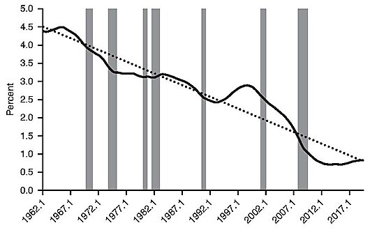
NOTE: Shaded gray areas are recessions as defined by the NBER.
SOURCES: Laubach and Williams (2003); New York Fed, www.newyorkfed.org/research/policy/rstar.
All signs therefore point toward an extended period in which interest rates are significantly lower than their average levels from the 1980s to 2000s. This means that the problem of the ZLB and the inability to push the FFR down in response to deteriorating economic conditions is likely to arise again. As a consequence, the Fed must move away from its conventional operating framework—for example, by significantly raising its inflation target, experimenting with negative rates, or more regularly using unconventional tools like QE as a substitute for conventional rate cuts at the ZLB. Which of these options should the Fed and other central banks choose?
The Problem of the ZLB and Policy Proposals to Avoid It
The macroeconomic models popular prior to the Great Recession—chiefly, New Keynesian dynamic stochastic general equilibrium (DSGE) models—were developed in the context of the Fed’s precrisis operating framework.1 These models feature one short-term interest rate (the policy rate) and abstract from the myriad debt instruments that are ubiquitous in modern economies. Decision rules for consumption and investment are derived from microeconomic decision problems. Nominal rigidities in the form of price and/or wage stickiness are introduced, giving rise to a Phillips curve-type relation between inflation and resource utilization. Monetary policy is characterized via some sort of rule, such as the famed Taylor (1993) rule, for the short-term policy interest rate.
The ZLB poses a substantial constraint for stabilization policy in these models. After all, there is only one policy instrument, and at the ZLB, this instrument is unavailable. Kiley and Roberts (2017) survey the costs of the ZLB in standard New Keynesian DSGE models and conclude that they are sizable. At the ZLB, the economy is much more susceptible to adverse demand shocks, and supply shocks can have nonintuitive effects on output and other aggregates (Cochrane 2017; Wieland 2019). Furthermore, at the ZLB, the economy can get stuck in a self-fulfilling trap of deflation and negative output gaps (Benhabib, Schmit-Grohe, and Uribe 2001).
Based on the prevailing view that the ZLB imposes substantial costs, many economists have pushed for policy changes meant to reduce both the likelihood and length of ZLB episodes. One popular proposal is to raise the Fed’s long-term inflation target. The logic behind such proposals is the celebrated Fisher relationship, which says that the nominal interest rate equals the real rate plus the rate of expected inflation. For a given real rate, higher expected inflation raises the nominal rate one-for-one. An inflation target of say, 4 percent instead of 2 percent, would therefore give the Fed and other central banks an average of two more percentage points of room for rate cuts before hitting the ZLB.2
A number of other economists have argued for wider implementation of negative interest rates as a policy tool (e.g., Kimball 2017; Rogoff 2017; and Agarwal and Kimball 2019). Conventional wisdom holds that the existence of currency paying a zero nominal return places a floor of zero on interest rates on other assets. Contrary to this wisdom, a number of central banks—with the Fed being a notable exception—have successfully implemented negative policy rates without much trouble, and at present, a large amount of sovereign debt is trading at mildly negative yields. Nevertheless, rates have not gone substantially negative anywhere in the world, and the existence of a zero-yielding substitute like cash, as well as other features of financial markets and institutions, likely puts a cap on just how far into negative territory rates can fall. For this reason, some economists have called for the (near) abolition of paper currency (e.g., Rogoff 2016).
The elimination of barriers on how negative nominal interest rates can fall might entail significant changes in central bank operating procedures, but if successfully implemented, it would render the problem of low rates moot—the Fed and other central banks could adjust policy by moving rates up or down as needed without regard for a binding floor, zero or otherwise. Increasing the inflation target by a few percentage points would give the Fed significantly more room to cut rates in the face of deteriorating economic conditions without having to worry about pushing rates into negative territory. Enabling deeply negative rates or increasing the inflation target would both represent a significant departure from Fed practice and would certainly entail some potentially large costs. But if the ZLB poses a substantial threat, perhaps those costs are worth incurring.
The Fed’s Unconventional Policy Actions
The large costs of a binding ZLB presuppose that central banks cannot do anything once policy rates have hit their floor. In actuality, neither the Fed nor the world’s other leading central banks sat idly by when short-term policy rates approached zero in the wake of the 2008 financial crisis and ensuing Great Recession. Rather, central banks engaged in a series of unprecedented policy actions meant to circumvent the ZLB. Taken together, these policy actions have been referred to as “unconventional” monetary policy.
In the middle of 2008, the total value of assets held by the Federal Reserve totaled less than $1 trillion. The majority of these assets were Treasury bills, notes, and bonds, and most of these assets were held to maturity.
The Fed’s first round of quantitative easing (or QE1) began in November 2008. The Fed initially began to buy $600 billion of agency mortgage-backed securities (MBS). The program was extended in early March 2009. The purchase of these securities was financed with the creation of bank reserves, on which the Fed had begun to pay interest in the fall of 2008.3 A second round of quantitative easing, or QE2, was announced in November 2010. It entailed purchasing another $600 billion of assets through the creation of reserves, though this time involved purchases of longer maturity Treasury securities rather than agency mortgage-backed securities. A third round of QE began in September 2012. This was announced as an open-ended program with a target volume of agency mortgage-backed securities purchases each month. Active balance sheet expansion ceased at the end of 2014. In between QE2 and QE3, the Fed engaged in the Maturity Extension Program (or “Operation Twist”), in which it sold short-maturity Treasury securities and used the proceeds to buy up longer-maturity Treasuries, in effect extending the maturity of its asset holdings without impacting the size of its balance sheet.
Figure 2 plots the magnitude of assets held on the Fed’s balance sheet dating back to 2003. Shaded regions denote periods of active QE purchases (QE1, QE2, and QE3). As noted above, prior to the Great Recession, the balance sheet was under $1 trillion. QE1, which was announced in the immediate wake of the Fed opening a number of emergency lending facilities, resulted in the Fed’s balance sheet being well over $2 trillion by mid-2010. QE2 brought the balance sheet to nearly $3 trillion and QE3 pushed the balance sheet to a peak of $4.5 trillion. This represented a nearly five-fold increase in the size of the Fed’s balance sheet in the span of six years.
FIGURE 2: THE FED’S BALANCE SHEET, 2003–2019
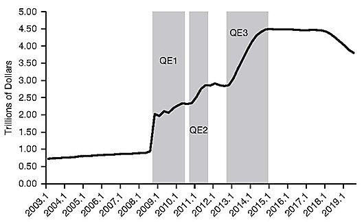
NOTE: Shaded areas denote periods of active QE programs.
SOURCE: St. Louis Fed, https://fred.stlouisfed.org/series/WALCL.
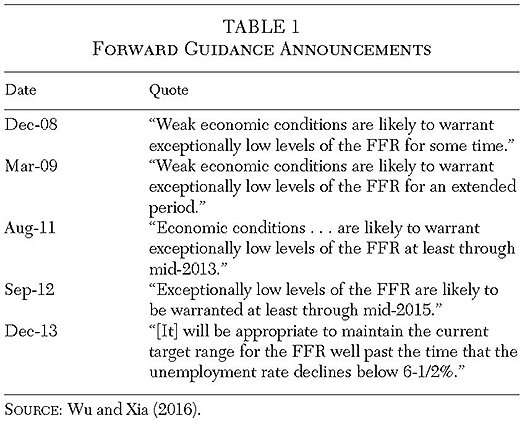
The other principal unconventional tool deployed by the Fed was forward guidance. Forward guidance involves telegraphing the intended path of policy rates after a period of low or zero rates. For an excellent overview of forward guidance and different types of forward guidance (e.g., Delphic versus Odyssean), see Campbell et al. (2012). By credibly signaling the intended path of future policy rates, forward guidance is meant to push down current long-term interest rates via the logic of the expectations hypothesis.
Less explicit forms of forward guidance had been employed by the Fed and other leading central banks prior to the Great Recession, but forward guidance became an even more important and explicit policy tool when the FFR hit its lower bound. Table 1 presents a selection of quotes characteristic of different types of forward guidance. As soon as the FFR hit the ZLB in December 2008, the Fed included in its minutes wording that indicated it anticipated that economic conditions would warrant a low FFR for some time into the future. It later adopted a more calendar-based type of forward guidance, being explicit about when it anticipated pushing policy rates back above zero. Finally, the Fed moved to target-based forward guidance, announcing explicit targets for the unemployment and inflation rates that would need to be hit before increasing the policy rate.
The Macroeconomic Effects of Unconventional Policies
There is a large literature that empirically studies the macroeconomic effects of QE.4 The majority of papers in this area find stimulative effects of QE, though findings differ somewhat concerning the magnitude and persistence of effects. Swanson and Williams (2014) and Gagnon and Sack (2018) provide overviews of these literatures. Some authors, notably Greenlaw et al. (2018), have questioned the persistence of QE, highlighting that the stimulative effects found in many event studies are quiet transient. Swanson (2018a) argues instead that QE effects are both strong and persistent and points to the special QE extension announcement from March 2009 as driving some of the transience results in the literature.
There is a similarly large literature on the effects of forward guidance, some of which actually predates the Great Recession (Gürkaynak, Sack, and Swanson 2007). For more recent work, see, for example, Campbell et al. (2012); Carvalho, Hsu, and Nechio (2016); or Campbell et al. (2017); or Campbell et al. (2017). These articles all find that forward guidance in particular, and central bank communication more generally, has important economic effects.
On balance, the literature on QE and forward guidance finds that unconventional policies had measurable economic effects that very likely lessened the severity of the Great Recession. See also the conclusion in Swanson (2018b). This coincides with several other empirical papers that show that the economy’s reaction to structural shocks during the ZLB period was not consistent with the predictions of standard New Keynesian macroeconomic models at the ZLB.5
A useful way to summarize the effects of unconventional policy actions is the so-called shadow rate. The shadow rate makes use of models of the term structure to infer a hypothetical value of short-term interest rates from the behavior of long-term rates as if there were no ZLB. A very popular shadow rate series is the one produced by Wu and Xia (2016). It is plotted in Figure 3 (dashed line) along with the effective FFR (solid line). The frequency of observation is quarterly and shaded regions denote periods of active QE purchases. The shadow rate reaches a nadir of nearly 3 percentage points below zero. This is suggestive that unconventional policy actions provided economic stimulus the equivalent of pushing the FFR significantly into negative territory.
FIGURE 3: SHADOW RATE AND EFFECTIVE FFR
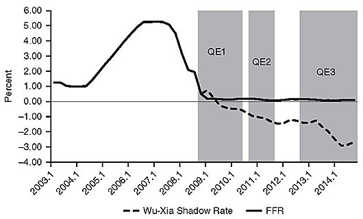
NOTE: Shaded areas denote periods of active QE programs.<
SOURCES: Wu and Xia (2016); Cynthia Wu, https://sites.google.com/view/jingcynthiawu/shadow-rates?authuser=0.
Modeling Unconventional Policy as a Substitute for the Policy Rate
The work cited above generally relies on reduced-form empirical techniques. In recent years, a number of researchers have worked to modify precrisis models to allow scope for unconventional monetary policy.
The efficacy of forward guidance in standard New Keynesian models has never been in doubt; indeed, the earliest work on the problem of the ZLB (e.g., Krugman 1998; Eggertsson and Woodford 2003) called for the expansive use of forward guidance during such periods so as to mitigate the economic costs of policy being constrained. More recently, other researchers have concluded that standard models predict that forward guidance is too powerful relative to what is observed in the data.6
Quantitative easing, in contrast, has no effects in standard macroeconomic models, where a form of “Wallace neutrality” holds (Wallace 1981). To provide scope for QE to matter, several recent papers explicitly model constrained financial intermediaries.7 In these models, endogenous leverage constraints arise, and central bank purchases or sales of assets can impact these constraints so as to endogenously affect credit spreads. Sims and Wu (2019a) show that exogenous shocks to QE can have impacts similar to a conventional policy rate change and, in a counterfactual Great Recession simulation, further show that a simple endogenous feedback rule for QE can largely mitigate the consequences of the ZLB.
The articles cited above employ medium-scale models with a number of different nominal and real frictions. Sims and Wu (2019b) instead develop a four equation version of the Sims and Wu (2019a) model that stays as close as possible to the benchmark three equation New Keynesian model of Galí (2008) while still allowing scope for QE. In a follow-up paper, Sims and Wu (2020) ask how much of the decline in the Wu-Xia shadow rate can be accounted for by the Fed’s QE purchases.
The starting point of their analysis is depicted in Figure 4, which plots the Wu-Xia shadow rate on the left axis along with the negative of the Fed’s balance sheet over the course of its QE operations on the right axis (measured in trillions of dollars). The frequency of observation is quarterly. The association between the shadow rate and the balance sheet is obvious and is suggestive, though of course not dispositive, of a causal link between the two.
FIGURE 4: SHADOW RATE AND FED BALANCE SHEET
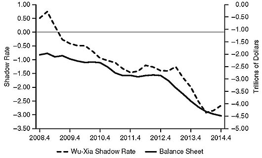
SOURCES: Wu and Xia (2016); Cynthia Wu, https://sites.google.com/view/jingcynthiawu/shadow-rates?authuser=0; St. Louis Fed, https://fred.stlouisfed.org/series/WALCL.
Sims and Wu (2020) use the four-equation model of Sims and Wu (2019b) to develop a model-implied shadow rate given the observed magnitudes of the Fed’s balance sheet expansion. Calibrated to U.S. data, they show that the observed increase in the Fed’s balance sheet over the course of its QE operations can account for more than two-thirds of the decline in the Wu-Xia shadow rate. This is shown in Figure 5, which plots their model-implied shadow rate (solid line) along with the observed shadow rate (dashed line).
FIGURE 5: SHADOW RATE AND MODEL-IMPLIED SHADOW RATE
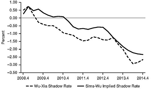
SOURCES: Wu and Xia (2016); Sims and Wu (2020).
The model-implied shadow rate of Sims and Wu (2020) lies above the actual shadow rate in almost all periods.8 This suggests, quite naturally, that QE alone cannot account for all of the observed stimulus from the Fed’s unconventional actions. After all, as noted in Table 1 and elsewhere in the text, at the same time that it was engaging in active bond purchases, the Fed was also using forward guidance. These results are in line with complementary work by Gagnon and Sack (2018), who argue that at peak, the Fed’s QE operations provided economic stimulus the equivalent of moving the FFR nearly 3 percentage points below zero.
Higher Inflation, Negative Rates, or Unconventional Policy?
Faced with a low and declining natural rate of interest, the Fed and other central banks must confront the reality that the precrisis operating framework of changing short-term policy rates needs some adjustment if monetary policy is to provide adequate stimulus in response to adverse economic shocks. Central banks must either significantly increase inflation targets so as to provide more room for traditional rate cuts, experiment with deeply negative rates and the requisite changes to the operating framework to make such actions feasible, or must regularly adopt unconventional actions such as QE and forward guidance whenever policy rates hit their lower bound.
We believe that the Fed and other central banks should opt for the latter of these options—unconventional policies, and in particular QE, ought to become a conventional part of central banks’ toolkits. Reduced form empirical studies, term structure models, and appropriately modified DSGE models all suggest that QE (and forward guidance) can provide adequate stimulus similar to conventional policy rate cuts. This conclusion aligns with work by Swanson (2018b) and Gagnon (2019). Even though there were serious concerns about potential side effects from QE at the time of its implementation (such as high inflation), few, if any, of these side effects have materialized. The massive run-up and slow but steady decline in the Fed’s balance sheet in the last year or two seem to have gone off without a hitch. We therefore see no practical political economy concerns with continuing to deploy QE in the future.
Absent some sort of behavioral bias, policymakers should be weakly better off with more tools at their disposal. It should therefore be the case that the ZLB nevertheless imposes some costs on policymakers in particular and on the economy more generally. Indeed, Sims and Wu (2019b) stress that QE is a good, albeit imperfect, substitute for conventional policy at the ZLB. Should, then, policymakers adopt one of the other two recommendations discussed in this paper to reduce the likelihood of the ZLB binding again in the future?
We are skeptical that raising the inflation target or experimenting more heavily with negative rates would do much good, and in fact could bring about other unintended consequences. The conquest of the high inflation of the 1970s and the credibility of the 2 percent inflation target were hard-fought victories that took years to achieve. Abandoning the 2 percent target in light of the recent ZLB episode therefore strikes us as short sighted. There are myriad potential costs of higher trend inflation. Coibion, Gorodnichenko, and Wieland (2012) find that the optimal inflation rate in New Keynesian models when taking the ZLB into account is quite small and remarkably close to the Fed’s 2 percent target. Ascari, Phaneuf, and Sims (2018) argue that increasing the trend inflation rate from 2 to 4 percent could be quite costly. Diercks (2019) provides a meta-study of articles examining the optimal long-run inflation target; the vast majority of these studies suggest that low or even negative inflation is optimal.
Negative rates have been implemented in a number of countries, although in no case have rates been pushed deep into negative territory. Eggertsson et al. (2019) document in Swedish data that the transmission from policy to deposit rates breaks down once policy rates turn negative and even show that policy rate cuts further into negative territory can lead to increases in lending rates. Similarly, Ulate (2019) theoretically emphasizes how negative policy rates can squeeze bank profitability, causing a partial breakdown of the usual monetary transmission mechanism. Similar forces are at work in Sims and Wu (2019a), whose model allows the interest rate on reserves to turn negative but imposes a ZLB on deposit rates. Negative rates can provide stimulus as a form of credible forward guidance but also work to erode the net worth of intermediaries, which has a contractionary effect. In their model, when central banks carry very large balance sheets financed via bank reserves, negative rates can even become contractionary, similar to the empirical findings in Eggertsson et al. (2019).
Conclusion
The recent experiences in the United States and other developed economies of policy rates being pushed to their lower bound are likely not one-off events. A low and declining natural rate of interest means that the Fed and other central banks will likely have to confront again the challenges of combating recessions with little or no room to cut short-term rates.
We argue, on the basis of a number of empirical studies as well as a literature based on quantitative macro models, that unconventional policies like quantitative easing and forward guidance may serve as effective substitutes for conventional rate cuts at the zero lower bound. Policy changes to reduce the incidence and severity of ZLB episodes, such as raising inflation targets or experimenting with deep negative rates, would impose additional costs and are therefore not desirable given the efficacy of policies such as QE.
References
Agarwal, R., and Kimball, M. S. (2019) “Enabling Deep Negative Rates to Fight Recessions: A Guide.” IMF Working Papers 19/84.
Ascari, G.; Phaneuf, L.; and Sims, E. (2018) “On the Welfare and Cyclical Implications of Moderate Trend Inflation.” Journal of Monetary Economics 99: 56–71.
Ball, L. M. (2014) “The Case for a Long-Run Inflation Target of Four Percent.” IMF Working Papers 14/92.
Bauer, M. D., and Rudebusch, G. D. (2016) “Monetary Policy Expectations at the Zero Lower Bound.” Journal of Monetary Economics 48 (7): 1439–65.
Benhabib, J.; Schmitt-Grohe, S.; and Uribe, M. (2001) “The Perils of Taylor Rules.” Journal of Economic Theory 96 (1–2): 40–69.
Campbell, J. R.; Evans, C. L.; Fisher, J. D. M.; and Justiniano, A. (2012) “Macroeconomic Effects of Forward Guidance.” Brookings Papers on Economic Activity 1: 1–80.
Campbell, J. R.; Fisher, J. D. M.; Justiniano, A.; and Melosi, L. (2017) “Forward Guidance and Macroeconomic Outcomes Since the Financial Crisis.” NBER Macroeconomics Annual 31: 283–357.
Carlstrom, C. T.; Fuerst, T. S.; and Paustian M. (2017) “Targeting Long Rates in a Model with Segmented Markets.” American Economic Journal: Macroeconomics 9 (1): 205–42.
Carvalho, C.; Hsu, E.; and Nechio, F. (2016) “Measuring the Effect of the Zero Lower Bound on Monetary Policy.” Federal Reserve Bank of San Francisco, Working Paper No. 2016-06.
Cochrane, J. H. (2017) “The New-Keynesian Liquidity Trap.” Journal of Monetary Economics 92: 47–63.
Coibion, O.; Gorodnichenko, Y.; and Wieland, J. (2012) “The Optimal Inflation Rate in New Keynesian Models: Should Central Banks Raise Their Inflation Targets in Light of the ZLB?” Review of Economic Studies 79 (4): 1371–406.
Debortoli, D.; Galí, J.; and Gambetti, L. (2019) “On the Empirical (Ir) Relevance of the Zero Lower Bound Constraint.” NBER Working Paper No. 25820 (May). Forthcoming in NBER Macroeconomics Annual 2019.
Del Negro, M.; Giannoni, M.; and Patterson, C. (2013) “The Forward Guidance Puzzle.” Federal Reserve Bank of New York Staff Report 574.
Diercks, A. (2019) “The Reader’s Guide to Optimal Monetary Policy.” Available at https://ssrn.com/abstract=2989237.
Eberly, J. C.; Stock, J. H.; and Wright, J. H. (2019) “The Federal Reserve’s Current Framework for Monetary Policy: A Review and Assessment.” NBER Working Paper No. 26002.
Eggertsson, G.; Juelsrud, R. E.; Summers, L. H.; and Wold, E. G. (2019) “Negative Nominal Interest Rates and the Bank Lending Channel.” NBER Working Paper No. 25416.
Eggertsson, G., and Woodford, M. (2003) “The Zero Interest-Rate Bound and Optimal Monetary Policy.” Brookings Papers on Economic Activity 1: 139–235.
Gagnon, J. (2019) “What Have We Learned about Central Bank Balance Sheets and Monetary Policy?” Cato Journal 39 (2): 407–17.
Gagnon, J.; Raskin, M.; Remache, J.; and Sack, B. (2011) “The Financial Market Effects of the Federal Reserve’s Large-Scale Asset Purchases.” International Journal of Central Banking 7 (1): 3–43.
Gagnon, J., and Sack, B. (2018) “QE: A User’s Guide.” Peterson Institute for International Economics Policy Brief.
Galí, J. (2008) Monetary Policy, Inflation, and the Business Cycle. Princeton, N.J.: Princeton University Press.
Garín, J.; Lester, R.; and Sims, E. (2019) “Are Supply Shocks Contractionary at the Zero Lower Bound? Evidence from Utilization-Adjusted TFP Data.” Review of Economics and Statistics 101 (1): 160–75.
Gertler, M., and Karadi, P. (2011) “A Model of Unconventional Monetary Policy.” Journal of Monetary Economics 58 (1): 17–34.
___________ (2013) “QE1 vs. 2 vs. 3 … : A Framework for Analyzing Large-Scale Asset Purchases as a Policy Tool.” International Journal of Central Banking 9 (1): 5–53.
Greenlaw, D.; Hamilton, J. D.; Harris, E.; and West, K. D. (2018) “A Skeptical View of the Impact of the Fed’s Balance Sheet.” NBER Working Paper No. 24687.
Gürkaynak, R.; Sack, B.; and Swanson, E. (2007) “Market-Based Measures of Monetary Policy Expectations.” Journal of Business and Economic Statistics 25: 201–12.
Hamilton, J. D., and Wu, J. C. (2012) “The Effectiveness of Alternative Monetary Policy Tools in a Zero Lower Bound Environment.” Journal of Money, Credit and Banking 44 (S1): 3–46.
Ireland, P. N. (2019) “Interest on Reserves: History and Rationale, Complications and Risks.” Cato Journal 39 (2): 327–37.
Kiley, M. T., and Roberts, J. M. (2017) “Monetary Policy in a Low Interest Rate World.” Brookings Papers on Economic Activity 48 (1): 317–96.
Kimball, M. S. (2017) “Next Generation Monetary Policy.” Journal of Macroeconomics 54 (A): 100–109.
Krishnamurthy, A., and Vissing-Jorgensen, A. (2011) “The Effects of Quantitative Easing on Interest Rates: Channels and Implications for Policy.” Brookings Papers on Economic Activity 2: 215–65.
___________ (2012) “The Aggregate Demand for Treasury Debt.” Journal of Political Economy 120 (2): 233–67.
Krugman, P. (1998) “It’s Baack! Japan’s Slump and the Return of the Liquidity Trap.” Brookings Papers on Economic Activity 2: 137–87.
Laubach, T., and Williams, J. C. (2003) “Measuring the Natural Rate of Interest.” Review of Economics and Statistics 4: 1063–70.
McKay, A.; Nakamura, E.; and Steinsson, J. (2016) “The Power of Forward Guidance Revisited.” American Economic Review 106 (10): 3133–58.
Rogoff, K. S. (2016) The Curse of Cash. Princeton, N.J.: Princeton University Press.
___________ (2017) “Dealing with Monetary Paralysis at the Zero Bound.” Journal of Economic Perspectives 31 (3): 47–66.
Sims, E., and Wu, J. C. (2019a) “Evaluating Central Banks’ Tool Kit: Past, Present, and Future.” NBER Working Paper No. 26040.
___________ (2019b) “The Four Equation New Keynesian Model.” NBER Working Paper No. 26067.
___________ (2020) “Are QE and Conventional Monetary Policy Substitutable?” International Journal of Central Banking 16 (1): 195–230.
Swanson, E. T. (2018a) “Measuring the Effects of Federal Reserve Forward Guidance and Asset Purchases on Financial Markets.” NBER Working Paper No. 23311.
___________ (2018b) “The Federal Reserve Is Not Very Constrained by the Lower Bound on Nominal Rates.” Brookings Papers on Economic Activity 2: 555–72.
Swanson, E. T., and Williams, J. C. (2014) “Measuring the Effect of the Zero Lower Bound on Mediumand Longer-Term Interest Rates.” American Economic Review 104 (10): 3154–85.
Taylor, J. B. (1993) “Discretion versus Policy Rules in Practice.” Carnegie-Rochester Conference Series on Public Policy 39: 195–214.
Ulate, M. (2019) “Going Negative at the Zero Lower Bound: The Effects of Negative Nominal Interest Rates.” Federal Reserve Bank of San Francisco, Working Paper No. 2019–21.
Wallace, N. (1981) “A Modigliani-Miller Theorem for Open Market Operations.” American Economic Review 71 (3): 267–74.
Wieland, J. F. (2019) “Are Negative Supply Shocks Expansionary at the Zero Lower Bound?” Journal of Political Economy 127 (2): 973‑1007.
Williamson, S. D. (2019) “The Fed’s Operating Framework: How Does It Work and How Will It Change?” Cato Journal 39 (2): 303–16.
Woodford, M. (2003) Interest and Prices: Foundations of a Theory of Monetary Policy. Princeton, N.J.: Princeton University Press.
Wu, J. C., and Xia, F.D. (2016) “Measuring the Macroeconomic Impact of Monetary Policy at the Zero Lower Bound.” Journal of Money, Credit and Banking 48 (2–3): 253–91.
Wu, J. C., and Zhang, J. (2019) “Global Effective Lower Bound and Unconventional Monetary Policy.” Journal of International Economics 118: 200–16.
About the Authors
Eric R. Sims is the Michael P. Grace II Collegiate Chair and Professor of Economics at the University of Notre Dame, and a Research Associate at the National Bureau of Economic Research. Jing Cynthia Wu is the Dillon Hall Associate Professor of Economics at the University of Notre Dame and an NBER Faculty Research Fellow.

This work is licensed under a Creative Commons Attribution-NonCommercial-ShareAlike 4.0 International License.