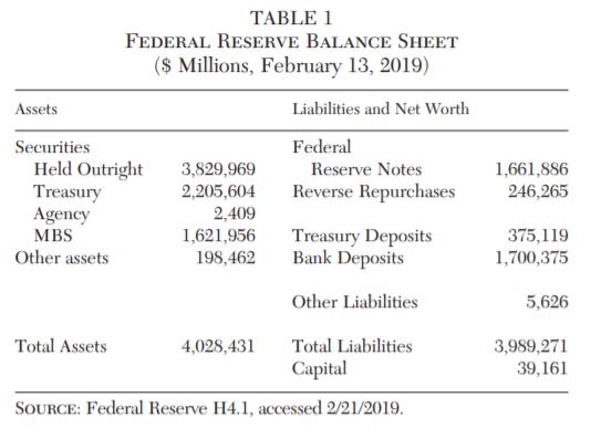
Ten years and $3.5 trillion of net asset purchases later, there is still no established answer to what effects the Fed’s unconventional policies produced or what the legacy of those polices will be. Yet, the footprint of those policies remains considerable. The Fed’s balance sheet (Table 1) is still close to $4 trillion and about 20 percent of nominal income, even after allowing some maturing investments to run off. The irony of quantitative easing (QE) is that its effects are hard to quantify. Prior to 2008, Fed officials lived in a comfortable world delimited to the basis point — actually to 0.25 percentage point — to which their interest-rate decisions always rounded. But unconventional policy, which includes adjusting guidance on interest-rate intentions and manipulating the size and composition of the central bank balance sheet, maps uncertainly into interest-rate expectations and liquidity preferences of investors.

In this article, I offer three perspectives on the Fed’s unconventional monetary policy. First, I draw on my work with Ben Bernanke in 2004, in which we framed expectations on the efficacy of unconventional monetary policy. The next section revisits those arguments.

Second, there is a cottage industry, including many contributions by Fed staff, in assessing the effects of unconventional policy.¹ This article employs finance theory to identify windows where views on policy are likely to be revealed and to look for relative price discrepancies among mostly similar instruments to parse policy effects. This is the popular solution to look under the lamp post for the missing item; I widen the window of observations to demonstrate that the effect proves ephemeral.

Third, this article exploits the enormous comovement among yields along the Treasury term structure. As has been known since Litterman and Sheinkman (1991), rates along the yield curve are well described by the current level, slope, and curvature of the yield curve. The fascinating feature is that any portion of the yield curve predicts other portions, a property I use to determine if the relationship between short and long rates changed pre- and post-QE. Long-term yields were a bit lower in the QE episode than short rates predicted but much more subsequently. Both approaches suggest that QE matters, but the effects are small relative to other macro forces pulling yields lower and likely to erode as the Fed’s relative footprint in markets shrinks over time.

The last section crosses over to the normative issue of the appropriateness of a large and lingering Fed footprint in markets. The revealed preference of policymakers is that they do not have sufficient confidence in market mechanisms or respect for the role of risk in directing the efficient allocation of resources. A healthier respect for both would place stricter limits on the extent to which a central bank leans against financial market volatility than was the case. The problem is that the precedent lowers the bar for future intervention and leaves the Fed operating under too large an ambit in our market economy.

What Were They Thinking?

The prior time that the Federal Reserve had a near brush with the lower bound of zero to the nominal policy rate was from 2002 to 2004.² The nominal federal funds rate touched the then unprecedented level of 1 percent, and replicating the ongoing “lost decade” of poor economic performance in Japan appeared a worrisome possibility. Among the work done at the time identifying policy alternatives was Bernanke (2002), Bernanke and Reinhart (2004), and Bernanke, Reinhart, and Sack (2004). When confronted by an adverse shock but pressed by the zero lower bound to nominal interest rates, a central bank could (1) signal to keep interest rates low for a sufficient time to pull longer maturity yields lower, (2) increase the amount of reserves beyond that necessary to push the policy rate to zero, (3) purchase assets in volume to influence their relative spreads, and (4) use administrative policies to subsidize lending.

The subject of this article is the third tool, also known as quantitative easing and large-scale asset purchases (LSAPs), although all these tools attempt to exploit one or more of four potential channels of influence on the economy. These channels are listed in the first column of Table 2. In particular, large-scale asset purchases might be seen as a demonstration of the willingness to keep interest rates low for a long time or “to do whatever it takes” in the memorable phrase of Mario Draghi, head of the European Central Bank. Assets are purchased through the creation of reserves and any money-multiplier effect may support lending and economic activity. If assets are imperfect substitutes, the purchase of some might influence risk premiums (in the manner discussed by Hanson and Stein 2015, and Krishnamurthy and Vissing-Jorgenson 2013).

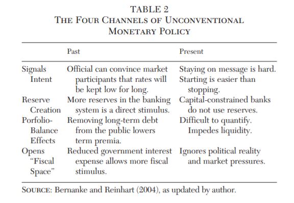
Moreover, the willingness of the central bank to purchase government securities might encourage politicians to issue more of them, providing fiscal impetus to an economy that was flagging (as discussed in Bernanke 2002). The diplomatic term for the collaboration of monetary and fiscal policy makers is creating “fiscal space.” The less delicate terms for QE that is never reversed are “debt monetization” and “financial repression.”

In retrospect, only two of these mechanisms got traction, and even those had drawbacks. Rate guidance had a material effect on rates, but sending a consistent message proved hard, especially in a committee setting (the Federal Open Market Committee or FOMC) when different views are expressed (Faust 2016). By way of example, for most of the stay at the zero lower bound from 2012 on (when rate guidance was first made explicit in the Summary of Economic Projections, SEP, of FOMC participants), investors viewed the stated policy direction as more hawkish than would actually be delivered. In addition, expressing the intention to keep rates at zero turned out to be easier than signaling the onset of tightening — it is easier to give than take away accommodation.

Large-scale asset purchases were associated with declines in yields, through some combination of forward guidance and portfolio-balance effects. The magnitude of such effects is hard to quantify and does seem to have had diminishing marginal effectiveness. On the other side of the ledger, market liquidity suffered as holdings became concentrated in official hands.

As for the two unconventional policies that never left the starting gate, reserves were created exactly when banks were risk averse and capital constrained, lessening the ability of banks to use them. Meanwhile, the Fed paid a market-related rate on excess reserves, lessening the incentive of banks to deploy them. As a result, reserves mostly sat on private balance sheets as excess reserves. That is, the money multiplier cratered. And politicians might have had the apparent ability to issue more debt but in many cases were unwilling to do so, in part on the fear of testing the tolerance of markets and the watchdogs at institutional financial institutions (as discussed in Reinhart, Reinhart, and Rogoff 2015).

The case for unconventional policy, then, rests on rate guidance and large-scale asset purchases. The former has long been part of Fed policy architecture, from the first publication of the SEP in 1977, the inclusion of a “bias” in the FOMC directive in the 1980s, the release of the FOMC statement in the 1990s, and expectations-shaping language such as “a considerable period” and “a measured pace” in the early 2000s (discussed in Lindsey 2003). The new wrinkle was the aggressive use of the balance sheet, QE, to be assessed quantitatively in the next section.

Quantifying Quantitative Easing

The Fed’s announcement of plans to add to its holdings of securities represents a natural experiment in how markets work and investors behave. To the extent that the news comes as a surprise, the repricing of long-lived assets reveals investors’ beliefs as to its effects. To the extent that they are concentrated in certain maturities, twists in turns in the yield curve may be informative about the role of guidance on the future path of rates versus portfolio-balance effects. We will follow these two paths in turn.

Looking under the Lamp Post

Event studies are an especially popular research strategy tracking price movements of long-lived assets in a narrow window surrounding an announcement (a small representative set is Gagnon et al. 2011, Krishnamurthy and Vissing-Jorgenson 2013, and Swanson 2018). An event is informative, however, only if the announcement is a surprise, which is difficult to guarantee when policymakers speak in public frequently and act in part in response to published economic data and prior market movements. Moreover, market capacity constraints might produce undershooting or overshooting of prices in brief time spans, and looking only at the announcement presumes there are no flow effects associated with actual purchases.

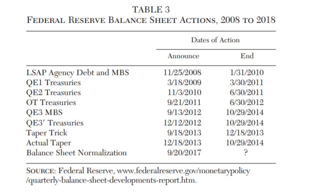
The analysis revolves around the seven FOMC announcements concerning asset purchases listed in Table 3. The first six involve the decisions to add to holdings and the seventh, “The Taper Trick,” occurred when the FOMC continued with asset purchases at the prevailing pace despite the predominant market view it would slow them. The last two rows provide the dates of reversals and are included for information’s sake. The window of observation was widened to one week (from the Friday to Friday bracketing the news) allowing time to observe the market absorption of QE news at the cost of adding non-QE noise. Table 4 provides the raw changes in financial market quotes for 19 assets. The choices are somewhat Treasury-security heavy because that is ground-zero for central bank policy intervention.

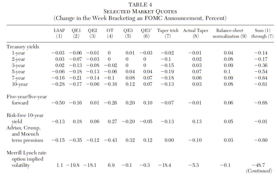
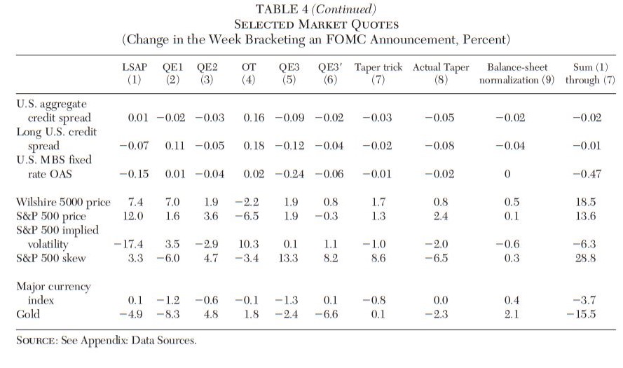
As is evident in the first six rows, LSAP news flattened the Treasury yield curve, consistent with signaling rates would be lower for longer as the front end was pinned at its zero lower bound and perhaps evidence of a portfolio-balance channel given that purchases skewed toward longer maturities.

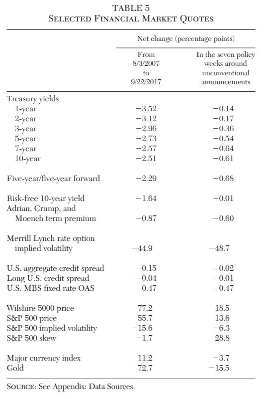
Across the seven easing actions, the 10-year yield fell 61 basis points, all of which came out of the estimated term premium, at least as judged by the proxy calculated by the Federal Reserve Bank of New York.³ Risk spreads mostly stayed unchanged, implying the change in Treasury yields passed onto borrowing costs. Mortgage-backed securities (MBS), which were a focus of Fed action, benefited particularly. LSAP announcements tended to curb the expected volatility of financial prices and to encourage risk taking in equity markets. The latter would follow both from a reduction in the discount rate and improved confidence about the economy. The fact that the dollar appreciated and gold prices fell probably indicate more weight should be put on the latter mechanism. These are squarely in line with other research and show that QE had market traction. However, two observations put this result in a more appropriate perspective.

Table 5 compares the net effect of the seven policy events (the second column) with the cumulative change from the start of the Fed’s expansionary efforts to the beginning of balance-sheet renormalization (the first column). The market mostly moved to provide financial accommodation over the period, but the bulk of the action occurred outside policy windows. QE mattered, but not that much.

Second, to see how lasting these effects were, the observation window was progressively widened one week at a time, calculating the change from the Friday before the announcement to up to 13 weeks later.⁴ Those changes were then regressed on a dummy variable identifying LSAP events, distinguishing between accommodative and restrictive announcements, and the change in the intended federal funds rate from 2006 to 2018 to soak up other policy noise. The first observation shown at the left in Figure 1 is the coefficient on the dummy marking out the seven accommodative LSAP announcements in the first regression for a one-week window.

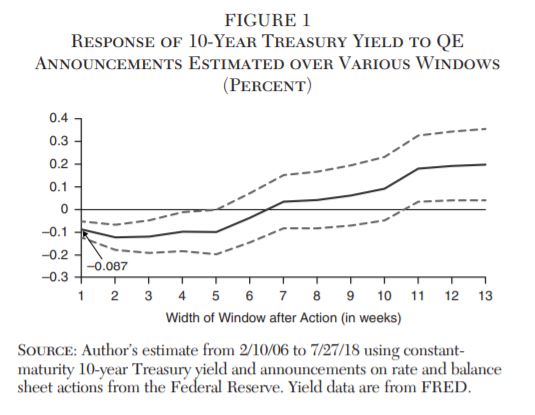
Arithmetically, this matches the result in Table 4, as seven events with an average effect of 8.7 basis points lowers the 10-year yield 61 basis points. The estimate differs from zero statistically and holds initially as the window is widened along the horizontal axis. However, five weeks on, there is no reliable reduction in yields. Put another way, with eight FOMC meetings scheduled regularly each year, an LSAP announcement at one of them left no reliable trace on the 10-year yield by the time of the next one.

Up and Down the Yield Curve

The second strategy is to exploit an extraordinary feature of the Treasury yield curve. As first shown by Litterman and Sheinkman (1991), the movement in yields across the term structure are well explained by three factors. As an even more important aid to intuition, those factors can be interpreted as the general level of yields, the slope of the yield curve, and its curvature. Moreover, those factors extrapolate across maturities, in that estimates gotten from one portion of the yield curve predicts yields at other portions of the yield curve that are of out of the estimation sample.

There are multiple ways to exploit this feature, but the stratagem here is to approach the yield curve from the front — use three factors derived from maturities up to two years to produce out-of-sample predictions of the 10-year yield in the QE period. The results are shown in Figure 2 and Table 6, where the factors — level, slope, and curvature — are defined as in Hamilton and Wu (2012), in which the 10-year yield is explained by rates up to two-years in maturity in the modern era of Fed communications up to the financial crisis, from 1994 to 2007. The predicted value (the dashed line) follows the actual (the solid line) over the sample period. Within the QE experiment period (the shaded LSAP area in the top of Figure 2), the yield is lower, by a little bit, as in the lower part of Table 6, consistent with the event study evidence that there is an effect but not a permanent one. Following the QE experiment, the 10-year yield systematically tracks materially below the prediction from short rates, about 1 percentage point, suggesting that other forces mattered more than the Fed’s balance sheet, which was shrinking relative to the amount of Treasury securities outstanding.

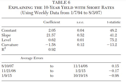
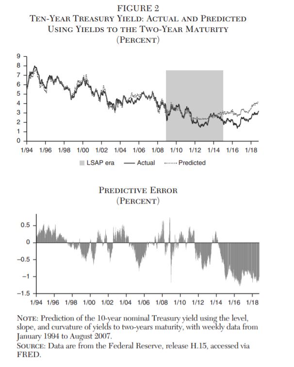
That is, long rates were relatively lower after the sunset of QE in the United States, not at its sunrise.

Two Cheers for Risk

Central bank actions in the financial crisis and thereafter were designed to reduce the volatility of financial prices. Sticking like glue to the effective lower bound on the nominal policy rate and offering explicit guidance about future policy kept investor uncertainty to a minimum about the rate to discount asset values. Large-scale asset purchases placed a floor on the prices of Treasury, agency, and mortgage-backed securities. Flooding the banking system with reserves ensured banks had safe collateral on their books. Deep down, this reflects a concern that an outsized deterioration in financial conditions (writ large across many assets) could trigger a more widespread deterioration, say perhaps as depositors run on a challenged institution that is solvent but illiquid or leads investors to dump assets in a fire sale.

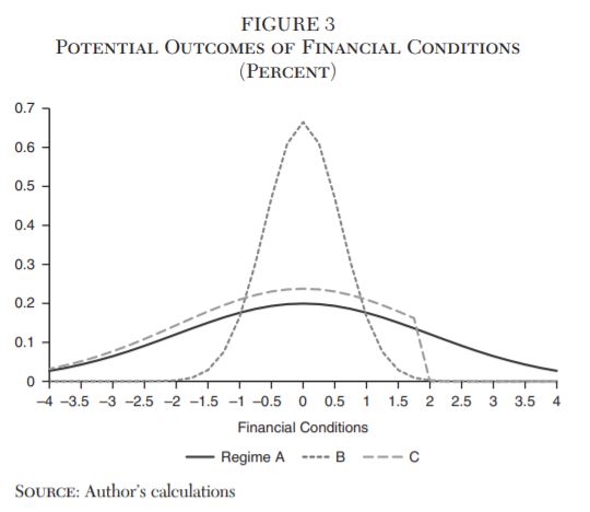
The idea is presented in Figure 3, which gives three possible distributions of overall financial conditions with different variances. In Regime A, which represents the environment within a financial crisis when investors were uncertain about the economic outlook and skittish toward risk, the area in the adverse right tail potentially creates an unacceptable chance of costly knock-on effects. The central bank response was to offer variance-damping reassurance (to get to Regime B) or outright price supports to cut off that tail (as in Regime C).

The titles of the memoirs of financial officials serving in 2008 and 2009 indicate considerable concern about those right-tail events and the imperative to act in the logical sequence of On the Brink, Stress Test, to the culmination in The Courage to Act.⁵ That these actions were appropriate in 2008 is far from settled (as discussed in Reinhart 2011) but at least the case for unconventional policy action in the United States was more compelling than it is for the continuation of those policies so long after the shock.

In particular, an outsized willingness to tamp down the volatility of financial prices neglects three important features of markets. First, not all volatility is unhelpful. The risk of capital loss leads investors to be more discriminating in asset choice and, over time, rewards those with more skill, a longer perspective, and a greater tolerance for risk. This encourages saving and directs capital to relatively more productive uses. Put the other way, by absorbing risk, the Fed lessened market discipline on institutions and investors. Moral hazard matters in its reward to indiscriminate risk taking and its distortion of capital decisionmaking.

Second, not all interventions are equal. Specific price supports (Regime C in Figure 3) shift the mean of expected outcomes, inflating asset prices. Included among the actors influenced are politicians, who may be encouraged to increase spending and cut taxes because there is little consequence for borrowing costs. To be sure, creating fiscal space may have been compelling in an economic recession, but it puts the long-term trajectory of government debt on a dangerous trajectory when low borrowing costs made U.S. deficits look more attractive in 2017–18. It also creates the political incentive for future monetization.

Third, by becoming a larger counterparty in specific markets, the Fed crowded out private-sector transactions. Indeed, some intermediation activity may disappear altogether, as was the case with the U.S. interbank market in the mid-1930s through the 1940s when the Fed tarried at the zero lower bound (Reinhart and Reinhart 2011). It is worth noting that, this time around, settlement volumes on Fed payment systems notched lower after 2008.⁶

These points combine to highlight the risk that overstaying market support may impair the efficiency of market mechanisms over time. But this is nothing new. In “Ironies of Automation,” Lisanne Bainbridge (1983) explained that people relying on machines may lose core competencies in the skills being automated. We no longer, in the modern setting, remember phone numbers because they are in our contact lists. Aside from inconvenience or embarrassment, the degradation of skills may impair the resilience of a system in response to unusual events. What do you do if the phone battery dies? More seriously, how can we keep pilots sharp enough to react in an emergency if most of their time in the cockpit is spent watching the autopilot work? How can we expect traders and investors to react reliably to shocks in the future if their past is one in which they have been protected by a benevolent central bank? This feature, by rendering markets less resilient, makes future official intervention more likely and self-justifying.

Conclusion

Unconventional monetary policy was an important driver of Treasury yields from 2008 to 2013, but not the only one nor the major one. Anyone asserting a more important role for the Fed has to explain why longer-term yields stayed low even as asset purchases reversed and short-term rates rose appreciably.

If the quantitative contribution of QE is limited, then the balance with its mostly uncounted adverse effects needs to be reassessed. An enlarged Fed presence influences market functioning and risk taking. Central to those effects are the extent to which the Fed absorbs risk that the private sector normally bore and disintermediates private parties in market activity.

The latter involves both sides of the Fed’s balance sheet. Risk absorption follows from the approximately $3.5 trillion of additional assets held by the Fed instead of the private sector. Purchased by creating the liability otherwise known as reserves, the Fed must find willing holders over time of its deposits or counterparties for its reverse repurchase facility. In both respects, this displaces traditional intermediation.

References

Adrian, T.; Crump, R. K.; and Moench, E. (2013) “Pricing the Term Structure with Linear Regressions.” Journal of Financial Economics 110 (1): 110–38.

Bainbridge, L. (1983) “Ironies of Automation.” Automatica 19 (6): 775–79.

Bernanke, B. S. (2002) “Deflation: Making Sure ‘It’ Doesn’t Happen Here.” Speech at the National Economists Club, Washington, D.C., November 21.

__________ (2015) The Courage to Act. New York: W. W. Norton.

Bernanke, B. S., and Reinhart, V. R. (2004) “Conducting Monetary Policy at Very Low Short-Term Interest Rates.” American Economic Review 94 (2): 85–90.

Bernanke, B. S.; Reinhart, V. R.; and Sack, B. P. (2004) “Monetary Policy Alternatives at the Zero Bound: An Empirical Assessment.” Brookings Papers on Economic Activity 2: 1–78.

d’Amico, S.; English, W.; López-Salido, D.; and Nelson, E. (2012) “The Federal Reserve’s Large-Scale Asset Purchase Programmes: Rationale and Effects.” The Economic Journal 122 (564): F415–F46.

Faust, J. (2016) “Oh, What a Tangled Web We Weave: Monetary Policy Transparency in Divisive Times.” Hutchins Center on Fiscal and Monetary Policy, Working Paper No. 25 (November 29). Washington: Brookings Institution.

Gagnon, J.; Raskin, M.; Remache, J.; and Sack, B. (2011) “The Financial Market Effects of the Federal Reserve’s Large-Scale Asset Purchases.” International Journal of Central Banking 7 (1): 3–43.

Geithner, T. F. (2014) Stress Test: Reflections on Financial Crises. New York: Crown.

Hamilton, J. D., and Wu, J. C. (2012) “The Effectiveness of Alternative Monetary Policy Tools in a Zero Lower Bound Environment.” Journal of Money, Credit and Banking 44: 3–46.

Hanson, S. G., and Stein, J. C. (2015) “Monetary Policy and Long-Term Real Rates.” Journal of Financial Economics 115 (3): 429–48.

Krishnamurthy, A., and Vissing-Jorgensen, A. (2013) “The Ins and Outs of LSAPs.” In Global Dimensions of Unconventional Monetary Policy, 57–111. Proceedings from the Kansas City Fed’s Jackson Hole Conference. Available at http://faculty.haas.berkeley.edu/vissing/jh.pdf.

Lindsey, D. E. (2003) A Modern History of FOMC Communication: 1975–2002. Washington: Board of Governors of the Federal Reserve System.

Litterman, R., and Scheinkman, J. (1991) “Common Factors Affecting Bond Returns.” Journal of Fixed Income 1 (1): 54–61.

Paulson, H. M. Jr. (2010) On the Brink: Inside the Race to Stop the Collapse of the Global Financial System. New York: Business Plan.

Reinhart, V. (2011) “A Year of Living Dangerously: The Management of the Financial Crisis in 2008.” Journal of Economic Perspectives 25 (1): 71–90.

Reinhart, C. M., and Reinhart, V. R. (2011) “Limits of Monetary Policy in Theory and Practice.” Cato Journal 31 (3): 427–39.

Reinhart, C. M.; Reinhart, V.; and Rogoff, K. (2015) “Dealing with Debt.” Journal of International Economics 96: S43–S55.

Swanson, E. T. (2018) “The Federal Reserve Is Not Very Constrained by the Lower Bound on Nominal Interest Rates.” NBER Working Paper No. 25123.

1 See, for instance, d’Amico et al. (2012), Gagnon et al. (2011), Krishnamurthy and Vissing-Jorgenson (2013), and Swanson (2018).

2 The time before was in the 1930s, as discussed in Reinhart and Reinhart (2011).

3 The framework is explained in Adrian, Crump, and Moench (2013). It is best not to overemphasize this parsing. An arbitrage-free term structure model infers the term premium through joint estimation of the price of risk and the present value of the path of the short-term interest rate. If the expected mean to which the short rate reverts falls suddenly, older observations will hold up the model’s estimate, which comes one-for-one at the expense of the term premium.

4 This methodology follows Swanson (2018) and, from here on, the focus is on the 10-year Treasury yield, the poster child for Fed action.

5 These were the titles of the memoirs, respectively, of Henry Paulson (2010), Timothy Geithner (2014), and Ben Bernanke (2015).

6 The data are found here: www.federalreserve.gov/paymentsystems/fedsecs_ann.htm.