Before 2008, the Fed could accelerate or decelerate inflation by expanding or contracting the monetary base and therefore bank reserves with open market operations and repo loans to dealers. Since 2008, however, the Fed has paid interest on excess reserves (IOER) equal to or even higher than the effective federal funds rate. As a result, the banks are awash with excess reserves that have zero opportunity cost, and the Fed has lost its primary mode of control over the price level and inflation.

In order to restore the Fed’s control over inflation, it is necessary that IOER be abolished. In doing so, however, it is also necessary to undo the post-2008 explosion of the base in order to prevent massive inflation.

Fed economists have recently invoked Milton Friedman’s 1969 essay, “The Optimum Quantity of Money” as providing justification for the Fed’s IOER policy. However, I shall show that strict application of this rule would leave the price level indeterminate in a fiat money world, and hence that it cannot be taken seriously as a monetary policy.

The zero lower bound (ZLB) issue has been used to justify many of the extraordinary measures the Fed has taken since 2008 as well as its interpretation of price stability as 2 percent inflation. This article shows that problem can be solved by temporarily targeting interest rates on loans with maturities longer than the six weeks implicit in the Fed’s current operating procedures, even with a 0 percent inflation target.

The Pre-2008 Regime

Prior to October of 2008, bank reserve deposits paid zero interest.¹ Banks normally held only a tiny inventory of excess reserves to meet withdrawals and adverse clearings, typically well under 0.5 percent of checkable deposits. The federal funds market efficiently allowed banks with surplus reserves and no immediate borrowing partner to lend them to banks that were short on reserves or were able to expand loans. The fed funds rate that banks charge one another for one-day use of reserves was typically well below the average rate banks got on somewhat risky customer loans that required close supervision, but represented the risk-adjusted opportunity cost to banks of marginal excess reserves.

Under this regime, if the Fed expanded the base and therefore excess reserves, banks would scramble to lend out any excess reserves beyond this small inventory to business or consumers who wanted the loans to make purchases they could not otherwise make, thereby driving up prices and at the same time temporarily driving down the fed funds rate.

Similarly, it could decelerate inflation by contracting the base, leaving banks with either precariously small excess reserves or an outright reserve shortfall. As banks contracted loans and thereby deposits to restore their reserves, businesses and consumers would spend less. At the same time, banks would temporarily bid the fed funds rate up.

Interest on Excess Reserves since 2008

Since October of 2008, the Fed has paid IOER at or slightly above the fed funds rate. During the same period, the Fed has more than quadrupled the monetary base though its QE I–III acquisitions of mortgage-backed securities (MBS) and Treasury securities. These acquisitions were financed mostly through the creation of new excess reserve balances. Thanks to IOER, however, banks have been in no rush to lend these funds out, and instead are content to just sit on them. The Fed in effect is now acting as a huge financial intermediary, borrowing reserve deposits from the banks at interest and lending them back to homeowners as mortgages or by transforming the maturity of the national debt.

This intermediation activity on the part of the Fed is not without adverse consequences, but has not in itself been inflationary, since IOER ensures that it is being financed with deposits that are savings instruments at the margin, rather than money per se. Thanks to IOER, the Fed is therefore essentially “rudderless” and unable to exert either inflationary or deflationary pressure on the economy.

When banks are awash with interest-bearing excess reserves, as they have been since 2008, there is little if any need for a federal funds market, since banks can earn interest simply by depositing surplus reserves with the Fed, and can obtain funds simply by withdrawing these deposits. To the extent there is a federal funds market, the fed funds rate should be essentially equal to the IOER rate. Indeed, the federal funds market has shrunk from over $300 billion in 2007 to barely $50 or $60 billion in recent years.

From late 2008 through November 2015, the IOER rate was only 0.25 percent and the fed funds rate itself was a little under 0.2 percent, neither of which is much different from zero—recall that the Federal Open Market Committee (FOMC) typically moves its fed funds target in multiples of 0.25 percent, which is therefore its estimate of the smallest perceptible increment to the rate. However, the Fed’s IOER policy in fact made a difference for banks’ willingness to hold reserves, since they could be confident that when market rates rose, IOER would rise with them, so that there never would be an opportunity cost to holding excess reserves. Since late 2015, the IOER and fed funds rate have indeed risen together, to 1.25 percent and 1.16 percent, respectively, by October of 2017.

The Fed’s Reckless Maturity Gambles

The Fed’s large-scale asset purchases represent financial intermediation rather than central banking—since they are being financed mostly by interest-bearing liabilities of the Fed that provide few if any monetary services at the margin.

Since the national debt is unlikely to be paid off any time soon, the Treasury prudently finances a large portion of it with long-term bonds, so as to lock in current long-term rates and protect taxpayers from even higher future interest rates. Moreover, because the Fed turns the bulk of its profits (or losses) over to the Treasury, its nonmonetary liabilities are essentially liabilities of the Treasury. The Fed’s purchases of long-term Treasury bonds with interest-bearing zero-maturity excess reserves therefore have essentially second guessed the Treasury’s prudent decision to borrow long with its own gamble to finance this substantial portion of the national debt with short-term borrowing instead. This is a decision that properly is the Treasury’s, not the Fed’s, and in any event the Fed is making the wrong decision.

Furthermore, by financing long-term mortgages with interest-bearing excess reserves, the Fed has taken the same reckless gamble that savings and loan associations (S&Ls) did in the 1960s and 1970s, and that led to the demise of most of the industry, not to mention the Federal Savings and Loan Insurance Corporation, during the 1980s. Long-term mortgages are a sound way to finance durable housing but should be financed by private intermediaries that issue long-term debt of comparable maturity. For all their faults, Fannie Mae and Freddie Mac have at least generally financed their mortgage portfolios with bonds of comparable maturity rather than with zero maturity savings accounts as did the now largely defunct S&Ls, and as now is being done by the Fed. In McCulloch (1981), I show that maturity transformation by financial intermediaries, or “misintermediation” as I call it, can upset the intertemporal equilibrium of the macroeconomy.

Unwinding IOER and the Fed’s Balance Sheet

Unfortunately, abruptly restoring IOER to zero would potentially be very inflationary, given the Fed’s bloated balance sheet, since it would be equivalent to suddenly quadrupling the base under the pre-2008 regime.

I have no easy solution to this predicament but recommend that the Fed immediately begin reversing its QE I–III acquisitions until the base is approximately back to its 2007 level, adjusted for nominal GDP growth, to approximately $1,130 billion. Treasuries have a very liquid market and can be sold as quickly as the Fed acquired them. Mortgage-backed securities are much less liquid, but at a minimum the Fed should immediately begin allowing them to run down to zero by not reinvesting in mortgages any interest or return of principal it gets from its mortgage portfolio. As it does this, I recommend that it should temporarily hold IOER at its present level, thereby gradually creating an opportunity cost to excess reserves as the base contracts and the fed funds rate eventually lift off above IOER. Then, when it has restored control of the base, it can lower IOER to zero and resume control of the fed funds rate by restoring a $10 billion to $50 billion repo loan balance with dealers as prior to 2008.

So long as currency pays zero interest, it has a clear opportunity cost (at least since early 2016 as nominal rates return to normal positive levels). Ultimately, the price level must equate the demand and supply of every monetary component, including currency. However, when banks are awash with zero-opportunity-cost excess reserves as at present, the Fed has no control over how much base drains from bank reserves into currency in circulation. This currency drain has been lethargic but steady, so that currency in circulation has almost doubled since 2007, while the nominal economy has grown only about 33 percent. While it is undoubtedly true that currency demand has been greatly increased since 2008 as a result of zero or near-zero interest rates, this situation cannot be expected to continue forever. This currency overhang should be cause for great concern.

Interest on Required Reserves

Interest on required reserves (IORR) is an entirely different matter than IOER. Before 2008, when IORR was zero along with IOER, reserve requirements acted as a modest excise tax on transactions deposits, and therefore gave banks a strong incentive to game them through the introduction of negotiable order of withdrawal (NOW) accounts, money market deposit accounts, and retail sweep accounts. These “near money” de facto transactions accounts have left the concept of M1 narrow money hopelessly muddled.

However, there is no particular reason to have a special excise tax on transactions deposits, aside from the Federal Deposit Insurance Corporation’s user fee for deposit insurance, since banks already pay income taxes on the income generated by their deposit-creation activities. I therefore recommend retaining IORR, setting it at, say, the average of the fed funds rate over the previous two weeks, or slightly lower.

One beneficial but little-noticed provision of Dodd-Frank is that it rolled back the anti-competitive 1933 prohibition of interest on demand deposits. Retaining IORR would therefore permit the consolidation of NOW accounts and money market deposit accounts, and therefore sweep accounts into a single interest-bearing demand deposit category, thereby greatly simplifying monetary statistics.

In order to give small banks relief from the implicit tax of zero-interest reserve requirements, Congress has mandated a 0 percent reserve requirement for the first $15.5 million of transactions accounts in any one bank, and only 3 percent for further transactions accounts up to $115.1 million. As a result, the average reserve requirement falls short of the 10 percent required for accounts in excess of $115.1 million, and depends on the accidental distribution of deposits between small and large banks. This uncertainty makes the bank expansion multiplier harder to predict than it otherwise would be. IORR makes this wild card in monetary policy obsolete, so that there now can be no objection to abolishing it.

Friedman’s Optimum Quantity of Money

Fed economists defending interest on reserves have recently made appeal to an unexpected quarter, namely Milton Friedman’s 1969 essay, “The Optimum Quantity of Money.”² As Ben Bernanke and Don Kohn (2016) put it, “Before the Fed paid interest on reserves, banks engaged in wasteful and inefficient efforts to avoid holding non-interest-bearing reserves instead of interest-bearing assets, such as loans.” New York Fed economists Laura Lipscomb, Antoine Martin, and Heather Wiggins (2017a, 2017b) make essentially the same argument, with explicit reference to Friedman’s essay.

This discussion takes me back to my graduate student days at Chicago, when Friedman’s essay had just come out, and one witty student had nicknamed it the “optiquan model.” “Optiquan” was written shortly after Friedman’s December 1967 American Economic Association presidential address, “The Role of Monetary Policy” (1968), in which he had refuted the notion, popularized by the Keynesians Paul Samuelson and Robert Solow, that positive inflation was beneficial to the extent that it reduced unemployment along a stationary Phillips Curve. He had convincingly argued instead that the Phillips Curve shifts up and down with expected inflation, so that the same “natural rate of unemployment” would arise at any sustained inflation rate.

But that left open the question: What inflation rate really is theoretically optimal under a pure fiat money regime in which the central bank is not constrained by a parity to gold or silver? (Recall that 1968–71 was precisely when the U.S. government, with Friedman’s approval, finally severed the dollar’s external link to gold.)

In “Optiquan,” Friedman argued that since fiat money is socially costless to produce, and since optimal inventory management induces money holders to incur real costs to keep down the forgone interest on their money balances, the first best optimum is to pick an inflation rate that drives the opportunity cost of money balances down to zero. One conceivable way this could be achieved would be by paying interest on all forms of money—both currency and demand deposits—at the same rate that could be earned on nonmonetary assets. A second conceivable method would be to engineer negative inflation just equal to minus the real interest rate that equated the nonmonetary demand and supply for credit, so that the nominal interest rate would be zero. In either case, agents would in theory hold such large money balances that at the margin they would be savings instruments and provide zero purely monetary services.

However, one big practical problem with the “optiquan model” that bothered me at the time and still does today is that it would leave the price level indeterminate: Friedman’s quantity theory of money predicts that the price level will gravitate to the level that equates the real value of the nominal money stock to the economy’s real demand for it. This requires (1) that there be a predictable real demand for an appropriately defined monetary aggregate and (2) that the central bank be able to control its quantity.

Friedman recognized that real money demand responds negatively to its opportunity cost, which, assuming money pays zero interest (as was the case for currency and all checking accounts outside New England before the 1980 Depository Institutions Deregulation and Monetary Control Act), would be the nominal interest rate on safe nonmonetary alternatives. He recognized that nominal rates fluctuate because of natural changes in real interest rates and also because of changes in expected inflation. However, inventory models of money demand predict that the money demand schedule is inelastic and therefore relatively steep at moderate nominal interest rates (when i is on the vertical axis and M/P is on the horizontal axis). Real interest rates are normally positive at all maturities, and must be positive at most maturities to prevent the price of land from being infinite. While inflationary finance is always fiscally tempting, deflation is fiscally unattractive, and therefore not an important long-run concern under fiat money, even by accident under a zero-inflation target. The demand for zero-interest money is therefore reasonably predictable as long as nominal rates are positive and inflationary expectations don’t drive them excessively high.

However, if the opportunity cost of money actually falls to zero, inventory models such as the famous Allais-Baumol-Tobin model (Baumol and Tobin 1989) predict that real money demand will be literally unbounded. Of course the resources of the economy are finite and money is not entirely costless—due to the risk of theft, loss, bank failures, or unanticipated inflation—so that money demand will never actually reach infinity, but the point remains that it becomes virtually indistinguishable from the horizontal axis over a wide range of values. This implies that an equally wide range of price levels will equate the supply and demand for money, and the quantity theory no longer predicts the price level, within this range.

Figure 1 illustrates the classical quantity theory of money when money pays zero interest, with moderate uncertainty as to the relevant parameters. The demand curve (dark gray) shows the inventory demand for real money balances M/P, with M/P on the horizontal axis and the nominal interest rate on the vertical axis. Because the money demand function is only known approximately, it is shown as a thick line. In equilibrium, the nominal interest rate will average out to the equilibrium real interest rate (r*) plus the inflation (π) that results from the central bank’s money growth policy. Since neither r* nor π is known with perfect certainty, their sum is depicted as a thick horizontal line (light gray). The intersection of the two curves determines real money balances and therefore the price level, but only imperfectly: given a nominal money stock M₀, the price level could be as high as P₂ or as low as P₁. So the price level is not determined precisely, but at least it’s reasonably bounded.

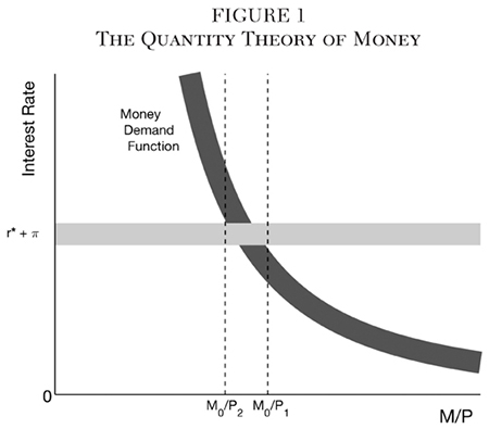
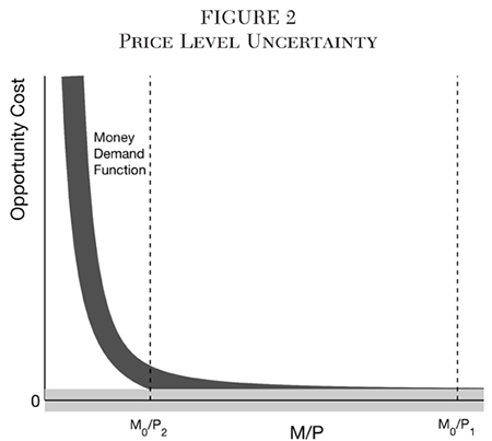
Figure 2 illustrates the inventory demand for money (dark gray) as a function of its net opportunity cost, net of any interest paid on money or real return from deflation. As the opportunity cost approaches zero, this schedule coincides with the horizontal axis, for all practical purposes. The thick horizontal line (light gray) depicts the approximately zero opportunity cost under the Friedman Optiquan deflation rule. Because the neutral real rate r* is uncertain and because the central bank cannot precisely control any deflation it engineers, this line again incorporates some uncertainty. Given a nominal money stock M₀, the price level is now indeterminate at any level between P₂ and P₁, and could be even lower than P₁.

In order for the value of a fiat money to be determinate, therefore, an appropriate monetary aggregate must have a clear and positive opportunity cost relative to nonmonetary assets. With all due respect to Friedman, his “optiquan model” is therefore just an interesting academic exercise that is in fact incompatible with the quantity theory. Its reasoning does argue against high-inflation policies, and does make a case for reducing the opportunity cost of at least the deposit component of M1 through interest on checking accounts. However, in order for the quantity theory to function, there must be a substantial aggregate controlled by the central bank that pays zero or at least greatly reduced interest.

The Zero Lower Bound Issue

The extraordinary measures the Fed has taken since 2008 have tied in with the ZLB issue as it affects the Taylor rule.³ This is an equation relating the FOMC’s federal funds rate target i* to a measure of anticipated inflation, Eπ, and, in its original formulation, the estimated percentage deviation of real output from its trend, ygap. The benchmark version of the equation, with coefficients as estimated by John Taylor (1993) on the basis of the Fed’s behavior in the 1980s and early 1990s, is

(1) i* = 1.0 + 1.5 Eπ + 0.5 ygap.

There is widespread agreement among economists that weak (i.e., less than 100 percent) feedback from expected inflation to i* was responsible for accelerating inflation prior to 1979, while strong (i.e., greater than 100 percent) feedback was responsible for bringing inflation down from double digits at the beginning of the 1980s to approximately 2 percent since 1990 (Clarida, Galí, and Gertler 2000). The actual coefficients depend on the Fed’s inflation target, on its estimate of the equilibrium real interest rate, and on how aggressively it wants to fight inflation and/or the output gap. Furthermore, the coefficients the Fed is using appear to have varied over time (Clarida, Galí, and Gertler 2000; McCulloch 2007). I shall use the above benchmark coefficients for the sake of illustration, with the understanding that the Fed may in fact choose to modify these coefficients. The output gap variable is problematic, but by definition averages out to zero, so that the long-run inflation implications of the Taylor rule lie entirely in the first two terms.

If inflation has been running at the Fed’s announced target of 2 percent and is expected to continue at this level, the above rule calls for a “normal” level of i* of 4 percent. This will be neutral with respect to inflation if the equilibrium or “natural” short-term real interest rate r* is 2 percent.⁴ If inflation falls to 0 percent and is expected from the time-series evidence to stay there while the estimated output gap is 0, the benchmark rule calls for an i* of 1 percent. This implies a real rate of 1 percent, which is less than its assumed equilibrium level of 2 percent, and hence would put upward pressure on inflation, driving it back toward the Fed’s announced target of 2 percent.

But if inflation falls to 0 percent and at the same time the estimated output gap is −4 percent, the benchmark rule calls for an impossibly negative i* of −1 percent, corresponding to a very stimulative real rate of −1 percent . Because of the ZLB on nominal interest rates, the lowest i* can ordinarily go is 0 percent. This would imply a real rate of only 0 percent, which would not be as stimulative as desired. This supposed ZLB threat has been used as a rationale for deliberately targeting a positive inflation rate in order to give the Fed some additional space to reduce nominal rates before hitting the ZLB, in spite of the Fed’s legislative mandate to stabilize prices. In 2012, the Fed in fact announced its intention to target 2 percent inflation, in part for this very reason.

We will see that this fear is unwarranted. But first, let us consider how the Taylor rule may be expected to operate when the ZLB is not binding.

The Taylor Rule When the ZLB Is Not Binding

Lowering the nominal interest rate y(m₀) on loans of maturity m₀ by Δi, while holding forward rates beyond m₀ constant, reduces the cost of borrowing to any maturity beyond m₀ by m₀Δi.⁵ Holding the public’s inflationary expectations constant, this makes current consumption less expensive relative to consumption at any maturity beyond m₀, thereby creating a proportionate excess demand for current output, financed by an equal and opposite temporary excess supply of money created by the Fed and the banks (see McCulloch 2012). This excess demand for current output generates proportionate inflationary pressure over and above expectations. The opposite is true for an increase in interest rates.

The federal funds rate itself is overnight (m₀ = 1/365), and so in itself has only negligible effect on the cost of credit or inflationary pressure. However, the FOMC meets only eight times a year, so that the effective m₀ of the Fed’s i* is 1/8 year on average, or about six weeks.⁶ The Fed typically (or at least prior to 2008) manipulates short-term rates through overnight loans to dealers via the repo market.⁷ However, if dealers can count on a particular value of i* continuing for the next six weeks, they can make a virtually riskless arbitrage profit by buying six-week Treasury bills and using them as collateral for a series of overnight loans, until the six-week T-bill rate equals i*. The Fed could achieve a very similar result without the intermediation of dealers by directly pegging the rate on T-bills maturing on or before the next FOMC meeting to i*.⁸ Since there is no reason for the credit premium on private loans to have changed, private loan rates will be similarly reduced, unless the Fed ends up holding a dominant fraction of all the maturing T-bills.

The direct effect of say a 100 basis point (1 percentage point) reduction in rates at even a 1/8 year maturity is still too subtle to create much inflationary pressure. However, if the market realizes this, it will recognize that conditions will most likely be similar to the present at the next FOMC meeting, and therefore that the FOMC will mostly likely choose a similar i*. This will create speculative demand for longer-term Treasury securities, financed by further short-term borrowing from the Fed at i*, until forward rates beyond 1/8 year on Treasury debt, and therefore private debt, reflect the probable trajectory of i*, as adjusted for the empirical term premium (see McCulloch 1975).⁹ This speculative demand for short-term loans from the Fed will magnify the direct and arbitrage demand, and can greatly increase the inflationary pressure of the low interest rate policy.

So long as the market is confident that the Fed will continue to fight high inflation (or below target inflation) with continuing tight (or easy) interest rate policy until inflation is back on target, there is therefore no need for the Fed to use “forward guidance” by announcing in advance a specific future interest rate target trajectory. Doing so is in fact counterproductive, because it may lead the Fed to feel bound to retain its promised interest rate trajectory despite conditions that in all likelihood will have changed somewhat, one way or the other. It is sufficient for the market simply to expect the Fed to aggressively follow a policy that will stabilize inflation as well as may be expected under a Taylor-type rule, with hands untied by the past.

Unexpected changes in interest rates on the part of the Fed necessarily generate unexpected capital gains or losses on loans of all maturities. However, the FOMC does well ordinarily not to directly intervene in forward rates beyond the date of its next meeting, since otherwise the decisions at the next meeting may generate capital gains or losses in the opposite direction. Only in the case when the zero lower bound (or a self-imposed above-zero lower bound) is binding should it venture into maturities beyond its next meeting.

The Taylor rule approach to monetary policy has the advantage over a money growth rule motivated by the quantity theory of money because it does not rely on knowledge or stability of the demand for real money balances. Yet it has the disadvantage, even in the absence of the ZLB issue, that it relies instead on the knowledge and stability of the equilibrium real interest rate r*. In practice, neither is fully known or stable, so that the monetary policymaker’s choice is between the less imperfect of two options.¹⁰

The Taylor Rule When the ZLB Is Binding

Now suppose that the ZLB on i* is binding. To take our earlier hypothetical example, suppose that experience with inflation and/or other variables would lead one to expect inflation to continue at 0 percent while ygap is −4 percent, so that the benchmark Taylor rule calls for i* = −1 percent, and the corresponding desired real rate of −1 percent is 3 percent below the natural real rate r* = 2 percent. However, the most it can lower the real rate before hitting the ZLB is by 2 percent, which would be only 2/3 of the desired stimulus. Nevertheless, it can still achieve the equivalent of a 3 percent reduction out to a six-week maturity, simply by lowering nominal rates to 0 percent and, therefore, the real rate to 0 percent out to nine weeks (3/2 of the six-week meeting interval) instead.

Doing this with no direct disturbance to forward rates beyond nine weeks would require the Open Market Desk to peg the interest rate on T-bills maturing within nine weeks of the current FOMC meeting to 0 percent, and to hold them there until the next FOMC meeting. At that time, the FOMC would then be free to continue the stimulus by moving the peg out another six weeks, or to alter the strength of the stimulus in either direction.

If the Fed, in our example, ends up holding a dominant share of all the outstanding T-bills maturing within nine weeks of the current meeting, it may have to supplement T-bill purchases with term repurchase agreements or term discount loans to insured commercial banks up to the same maturity date, in order to appropriately impact rates on private loans that compete with Treasuries.

If the Fed wished to avoid potential complications of 0 percent interest rates, it could alternatively achieve the same stimulus, in our example, by pegging rates at say 1 percent (a “unit lower bound,” so to speak), so that the real rate is 1 percent below the natural rate of 2 percent rather than the desired 3 percent, out to 18 weeks (6 weeks × 3 percent / 1 percent) from the current meeting.

Thus, although the ZLB may require some adjustment of procedures, it does not in itself prevent the functioning of the Taylor Rule. In particular it does not justify the adoption of a positive inflation target in lieu of price stability. For example, if the Fed chose to target 0 percent inflation while retaining the 1.5 coefficient on expected inflation, the 0.5 coefficient on ygap, and the 2 percent assumption on r*, it would have to raise the intercept in the Taylor rule to 2.0. Then if accidental deflation led the public to expect inflation to be −1 percent, while ygap was −4 percent, the rule would call for i* = −3 percent, or 4 percent below r*. An equivalent stimulus could be achieved with a real rate of 1 percent (1 percent below r*), at a maturity of 4 × 1/8 year, or 1/2 year. A “unit lower bound” as discussed in the preceding paragraph would not give the Fed much room to maneuver, but if it chose a 0.25 percent minimum Fed funds rate, which would correspond to a real rate of 1.25 percent with 1 percent expected deflation, or 0.75 percent below r*, it could achieve the desired stimulus with m₀ = 2/3 year.

References

Baumol, W., and Tobin, J. (1989) “The Optimal Cash Balance Proposition: Maurice Allais’s Priority.” Journal of Economic Literature 27 (3): 1160–62.

Bernanke, B. S., and Kohn, D. (2016) “The Fed’s Interest Payments to Banks.” Ben Bernanke’s blog, Brookings Institution (February 16).

Clarida, R.; Galí, J.; and Gertler, M. (2000) “Monetary Policy Rules and Macroeconomic Stability: Evidence and Some Theory.” Quarterly Journal of Economics 115: 147–80.

Fisher, I. ([1930] 1974) The Theory of Interest. New York: Augustus M. Kelley.

Friedman, M. (1968) “The Role of Monetary Policy.” American Economic Review 58: 1–17.

__________ (1969) “The Optimum Quantity of Money.” In M. Friedman (ed.) The Optimum Quantity of Money and Other Essays. Chicago: University of Chicago Press.

Lipscomb, L.; Martin, A.; and Wiggins, H. (2017a) “Why Pay Interest on Required Reserve Balances?” Liberty Street Economics blog, Federal Reserve Bank of New York (September 25).

__________ (2017b) “Why Pay Interest on Excess Reserve Balances?” Liberty Street Economics blog, Federal Reserve Bank of New York (September 27).

McCulloch, J. H. (1975) “An Estimate of the Liquidity Premium.” Journal of Political Economy 83: 95–119.

__________ (1981) “Misintermediation and Macroeconomic Fluctuations.” Journal of Monetary Economics 8: 103–15.

__________ (2007) “Adaptive Least Squares Estimation of the Time-Varying Taylor Rule.” Available at www.econ.ohio-state.edu/jhm/papers/TaylorALS.pdf.

__________ (2012). “The Theory of Money and Credit.” NYU class notes (September). Available at https://newclasses.nyu.edu/access/content/user/jhm406/MoneyAndCredit.pdf.

__________ (2015) “The Taylor Rule, the Zero Lower Bound, and the Term Structure of Interest Rates.” In W. Barnett and F. Jawadi (eds.) Monetary Policy in the Context of Financial Crisis: New Challenges and Lessons. Bingley, U.K.: Emerald Press.

__________ (2017a) “The Rudderless Fed.” Alt-M blog (September 8). Available at www.alt-m.org/2017/09/08/the-rudderless-fed.

__________ (2017b) “Optiquandary: A Practical Problem with Friedman’s ‘Optimum Quantity of Money.’ ” Alt-M blog (November 30). Available at www.alt-m.org/2017/11/30/optiquandary-practical-problem-with-friedmans-optimum-quantity-money.

Selgin, G. (2017) “Testimony before the U.S. House of Representatives Committee on Financial Services, Monetary Policy and Trade Subcommittee, Hearings on ‘Monetary Policy versus Fiscal Policy: Risks to Price Stability and the Economy.’ ” (July 20). Available at https://financialservices.house.gov.

Taylor, J. B. (1993) “Discretion versus Policy Rules in Practice.” Carnegie-Rochester Conference Series on Public Policy 39: 195–214.

¹The following two sections draw heavily on McCulloch (2017a). See also Selgin (2017).

²This section is based on McCulloch (2017b).

³The following three sections correct certain errors in McCulloch (2015). The present article therefore supplants the corresponding sections in that article.

⁴The equilibrium real interest rate is that determined in the absence of a monetary disequilibrium by the supply and demand for saving, as in the “loanable funds model” of Irving Fisher ([1930] 1974). This is equivalent to Knut Wicksell’s “natural rate of interest,” as discussed by Friedman (1968).

⁵If y(m) is the continuously compounded nominal zero-coupon yield to maturity m, the discount factor δ(m) = exp(−m y(m)) is the current price of $1 payable at maturity m, and f(m) = −d/dm log δ(m) = y(m) + m y′(m) is the instantaneous forward interest rate at maturity m. Changing y(m₀) by Δi while holding f(m) unchanged for all m > m₀ will change log δ(m) by −m₀ Δi for all m ≥ m₀.

⁶The FOMC has occasionally changed its fed funds target between regular meetings, via an emergency conference call meeting, but such events are rare enough to ignore for present purposes.

⁷A repurchase agreement, or repo for short, is in effect a short-term loan secured with Treasury securities. Legally, the effective borrower sells a security to the effective lender, and at the same time agrees to buy it back in the near future at a slightly higher price, reflecting the effective interest rate. In practice, “triparty” repos are often used, in which a custodial third party bank is the legal owner of the collateral securities throughout.

⁸Historically, maturing Treasury bills typically yield approximately 90 percent of the effective federal funds rate. This is presumably due to their exemption from state and local income taxes, in addition to their greater freedom from default risk. The fed might therefore in practice target a T-bill rate equal to about 90 percent of its fed funds target. In the text I have abstracted from this minor technicality.

⁹The present article abstracts from the term premium and assumes that the (log) expectations hypothesis is valid.

¹⁰In an open economy with a fiat currency, a third option is to fix the exchange rate to a foreign fiat currency. However, this is superior only if the foreign country has solved the problem of stabilizing the value of its own currency.