Clearly, doing away with paper currency entails important tradeoffs that must be considered by policymakers. Whereas currency might reduce the costs of tax evasion, corruption, and drug trafficking, and cause discomfort to central bankers, it has a long history as a beneficial and popular means of legitimate payment. Whether we should support proposals to eliminate large-denomination banknotes or circulating currency altogether depends on whether, overall, the benefits of doing so exceed the costs. Does ditching currency improve social welfare?

I argue that there are two essential dimensions to any approach that seeks an answer to this question. First, the framework for analysis must be one of general equilibrium—all channels through which such a major policy change affects economic incentives and behavior, both direct and indirect, must be considered. Second, the analysis must be quantitative. Pointing out the potential responses to the policy change can give us an understanding of the qualitative nature of the effects of demonetization, but only gets us so far. Understanding their overall effect on human well-being requires assessing the magnitudes of the tradeoffs, how big the costs and benefits are. Formal models of the overall economy are needed to achieve this understanding.

The aim of this article is to make an initial pass at measuring the welfare effects of currency elimination in the United States using the tools of macroeconomic theory. I rely on a standard dynamic general equilibrium model extended to allow households to avoid taxes by not reporting income, where holding and using money helps toward that end. Money in the model also serves to reduce the costs of legal transactions in consumer goods. Thus, the model, in a stylized but general way, captures the demand for holding money both for legitimate purposes and to facilitate tax evasion. For tractability, my model does not distinguish currency from other forms of transactions media; the model’s analog to currency demonetization is the analytical assumption that government monetary authorities can control how productive money is as a tax evasion device. In the model, reducing the productivity of money for tax evasion is tantamount to lowering the share of paper money in the nation’s overall money supply. I use this framework to illustrate the basic macroeconomic tradeoffs that eliminating currency would involve, and to quantitatively predict the overall effects on welfare.²

With only mild apologies, I set up the model to focus on tax evasion as the sole means by which paper currency can be abused, and ignore the many other illicit uses of cash, such as drug trafficking, prostitution, money laundering, and corruption. For many of these activities it would be straightforward to generalize the model to account for their role, but for my purposes doing so would excessively complicate things. Perhaps more importantly, though, tax evasion in the United States is, according to Rogoff (1998: 59), “truly massive” and is an important, if not the most important, underground use of cash in the United States. Thus, the costs and benefits of policies to diminish tax evasion—like currency demonetization— are relevant and worth studying. At the same time, while tax evasion introduces its own distortions and inequities, unreported income can also be an efficient response to tax distortions and can create incentives for work and production, which affects the cost-benefit calculus. It is also not clear how to appropriately incorporate some illicit activities, like the drug trade and prostitution, into the analysis when simply legalizing these activities would probably be a first-best solution. Finally, the model in this article has nothing to say regarding the negative-interest-rate argument for eliminating cash; I simply note that there are many ways to pay negative interest rates on cash, as described by Kimball (2017) for example, so that the potential benefit of currency elimination has less importance for monetary policy than its supporters might suggest.³

Here is a rough sketch of the relevant interactions in the model. Holding currency, by encouraging tax evasion through unreported income, reduces the effective income tax rate of the average household. Thus, cash holdings increase after-tax returns to labor and capital, which in turn increase the supply of inputs to firms, increase output, and increase the tax base. Whether tax revenues rise with money and tax evasion depends on the relative strength of the opposing movements in the effective tax rate and the tax base. Government spends resources on public goods, which directly improves welfare and which also increases factor productivity (think of infrastructure expenditures, like roads). Government policy that reduces the effectiveness of money as a tool for tax evasion—like eliminating large-denomination notes—can therefore have complicated effects on welfare by affecting work (and leisure), production, consumption, tax revenues, and government spending. The model accounts for all of these effects and feedback loops. The model also accounts for the likelihood that policies to eliminate cash or large-denomination notes also unavoidably negatively affect the ability of money to reduce transactions costs for legitimate purposes.

There is a large literature on tax evasion; for surveys see Slemrod (2007) and Alm (2012). Balafoutas et al. (2015) is a recent attempt to measure the costs of tax evasion, while Mazhar and Mon (2017) empirically consider the impact of the underground economy and tax evasion for developing and developed economies. Gordon (1990) is an early theoretical effort to examine the role of currency for tax evasion but is not a general equilibrium analysis. Camera (2001) moves in the right direction with a search-theoretic, general equilibrium framework that specifically models interactions between illegal activities and alternative media of exchange. Yet his model is complex and there is no quantitative welfare analysis. Much work in this area uses currency demand to estimate the size of the underground economy, as in Cebula and Feige (2012). This work is useful, but none of these papers or those cited in the surveys provide direct estimates of welfare effects of currency demonetization, which motivates my paper.

Without question this model is too stylized and restrictive to provide confident policy advice. For example, not only do I ignore other factors besides tax evasion where the use of currency can impose costs to society, but I also do not account for other exchange media that can aid tax evasion. Yet the model remains a reasonable way to examine the questions at hand if we simply assume that alternative media reduce the capability of the government to restrict cash’s productivity for tax evasion. The main strength of the model is that the general equilibrium effects are coherent and can be quantified. To obtain magnitudes, I calibrate the model’s parameters to plausible values and compute the implications for the steady-state values of consumption, employment, output, and welfare. Ignoring short-run dynamics is another important shortcoming of the article that needs to be dealt with in future work.

As will be seen below, for the benchmark parameterization, as well as for some alternatives, social welfare goes down when money’s tax-evasion productivity falls owing to government action on the order of magnitude of what a large-note demonetization in the United States might entail. The loss in welfare from the resulting increased tax burden and reduction in output and consumption is not offset by the gains from an increase in public goods and infrastructure spending. Nonetheless, this finding is sensitive to the calibration and the model specification, so I make no claims here on the optimal policy stance. The modest goal of this paper is to describe a feasible approach for assessing the potential welfare gains to society of eliminating currency.

The Model

I imagine an economy consisting of many identical households, many identical profit-maximizing firms, and a government sector. Households earn income by supplying labor and physical capital to firms in competitive factor markets; firms in turn use these inputs to produce a consumer good based on a common production technology. The produced good is sold by firms to households and the government sector in competitive markets as well. All actors in this economy take prices—wages, interest rates, and the overall price level—as given when making allocation decisions. These prices adjust to ensure that input and output markets clear, households maximize their utility, firms maximize their value, and the government taxes and buys its share of output, all obeying the economy’s overall resource constraint.

Households are forward-looking and infinitely lived, and have perfect foresight about the future.⁴ They maximize lifetime utility, derived from current and future consumption of the produced good and from leisure, subject to a resource constraint. This constraint depends on households’ lifetime flow of income generated by supplying labor and capital to firms, for which they earn wages and profits net of income taxes paid to the government sector, and the ability to accumulate new capital in financial markets. Households hold and accumulate real (fiat) money balances because cash reduces transactions costs incurred when consumer goods are purchased and serves as an input into a “tax evasion” technology (more on this below). Money is also subject to storage costs, which are increasing in the quantity of money. Households’ utility maximization ultimately determines the demand for consumption, the supply of labor (which is the households’ only alternative use of time besides leisure), the demand for money, and the accumulation of capital through saving, all as they evolve over time.

Firms produce output according to a constant-returns-to-scale production technology. Because firms hire labor and rent capital from households, maximizing the value of the firm (discounted lifetime profits) is tantamount to maximizing profits each period. This objective generates firms’ demand for labor and capital and determines the supply of consumer goods. The model’s equilibrium is the predicted outcome of household and firm interaction in competitive markets, as prices ensure that supply and demand are equal in all markets. This outcome determines quantities for household consumption, employment, capital accumulation and total output of the produced good (GDP).

The government sector purchases a share of produced goods, financed by collecting lump sum and flat rate income taxes, and by issuing new nominal money balances, which provides seigniorage.⁵ To simplify, I assume that the government sets the nominal money supply to grow at a constant rate, and ignore countercyclical monetary policy that is not needed in a full-employment steady state. The government, without cost, converts its purchases of produced goods to public goods that provide utility directly to households and increase the productivity of labor and capital. Equilibrium in the model also requires that the real supply of money provided by the government equal the demand for money arising from households’ optimal decisions, and that the government always satisfy its budget constraint.⁶

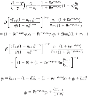
To better understand the model and to quantify its predictions, it is necessary to formalize it. Exposition of the model’s formal structure is aided by ignoring prices and treating the competitive economy as being directed by a fictitious central planner who chooses optimal consumption, employment, capital accumulation, money holdings, and output given full information about preferences and technology.⁷ The formal model is given by the following equations:

Equation (1) is the representative household’s lifetime utility function, which depends on consumption (c), leisure (1 − n, where n is labor supply given a unit time endowment), and the provision of public goods by the government (g_t). Future utility is discounted to the present at the rate of time preference, ρ. The household chooses time paths for c_t, n_t, k_t+1 (physical capital) and real money balances (m_t = M_t /P_t, where M is the nominal stock of money, P_t is the price level, and π_t = (P_t − P_t−1)/P_t−1 is the inflation rate) to maximize (1) with respect to the sequence of constraints in equation (2), presumed to hold for each period in the planning horizon. In equation (2), i_t is gross investment in physical capital, θ is the constant rate of price level inflation set by the government, y_t is total output of the produced good (GDP), T_t are lump sum taxes, τ(m_t) is the effective income tax rate where money can be used to shield taxable income, v(m_t) is the proportion of consumption expenditures used up in transactions, and the last term is a quadratic storage cost function for currency. Equation (3) is the production function that I incorporate directly into the household’s constraint owing to the central planner assumption: α is the elasticity of output with respect to the capital stock, and a is the elasticity of output with respect to government spending.⁸ The final equation is the government’s budget constraint, which shows that government spending is financed by income taxes and money growth. All lowercase variables, except labor, are real (as opposed to unit of account) values and measured in terms of the consumer good. Labor is simply the number of hours worked.

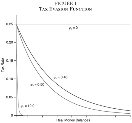
The important innovation in the model, due to Rogoff (1998) and essential for the aim of this article, is the effective tax rate function, τ (m_t). I restrict the function so that as m increases the effective tax rate falls, although it is assumed to fall at a declining rate. The function accounts for the potential value of cash as an anonymous transaction medium that enables households to underreport income to the government, which reduces their effective tax rate. I parameterize the function to be τ (m_t) =

e^−φτmt, where φ_τ > 0 and is the constant statutory income tax rate. φ_τ is the semielasticity of the household’s effective income tax rate with respect to its holding of real money balances, and can be thought of as the marginal value of money for tax evasion.

The key parameter of the analysis is φ_τ. I assume that the government sector has some control over its value. A policy that reduces φ_τ will make money less valuable as a means for avoiding taxes, and will also lower money’s value in reducing legitimate transactions costs. I implement the latter assumption by making v(m_t) depend negatively on φ_τ . Reducing φ_τ is the model’s analog to proposals to eliminate currency or large-denomination banknotes, and is the policy change I examine in this article.

What does the model predict will happen, economy wide, under such a policy? A decrease in φ_τ increases the effective tax rate for a given level of cash holdings and thus increases tax revenues for a given tax base. All else the same, government spending rises with the increase in tax revenues, which will increase household welfare through additional public goods and output through enhanced factor productivity. At the same time, however, there is downward pressure on output because, since the return to labor and capital falls with the increase in effective tax rates, labor and capital inputs fall. More resources are also wasted through higher transactions costs for consumption. As employment falls and leisure rises, welfare increases. But as output falls, so do consumption and welfare. Also, the equilibrium response of tax revenues, and therefore government spending, is ambiguous because of the offsetting movements of tax rates and the income tax base. The ultimate effects on output, consumption, and welfare are complex and subtle, and depend on the magnitudes of the model’s parameters. The value of a numerical simulation, performed in the next section, is to quantitatively evaluate these general equilibrium effects on the basis of plausible calibrations of the model.

Clearly, the model is highly stylized and misses important channels through which altering the composition of the money supply, by eliminating currency, will affect economic activity and welfare. However, the mechanisms built into this model are general enough to shed light on the channels of influence. For example, in the model I have considered only one type of money—currency—and have assumed away bank deposits and the importance of the composition of the money supply. However, interpreting money in the model as M1 (currency and checkable deposits) would simply scale down the value of φ_τ, and eliminating currency altogether could still be interpreted as a reduction (perhaps of smaller magnitude) in money’s tax evasion elasticity. Similarly, the existence of alternative tax evasion media, like gold or bitcoin, could be accommodated by suitable scaling of φ_τ. In the end, richer models than the one used here are needed to confidently understand the costs and benefits of currency elimination in the United States. However, the simple model of this paper is a reasonable start.

Simulation

Given specific functional forms, the model above can be solved for the variables of interest in a straightforward manner using standard techniques. I ignore transitional dynamics and focus on the model’s steady state—the time-invariant equilibrium quantities of household consumption, employment, capital stock, money holdings, and government expenditures and their implications for household welfare, to which the system converges over time. These values are functions of the model’s parameters, which I calibrate to force the steady state to roughly match U.S. experience. I then compare initial steady-state magnitudes to the new steady state for a policy-induced change in parameters. In particular, I consider the effects on steady-state quantities and welfare of a reduction in the value of money for tax evasion, which I take to proxy for currency or large-note elimination. The appendix provides technical details about the model, its solution, and its steady state. The appendix also reports the calibrated parameter values used to simulate the model.

Figure 1 illustrates the form of the model’s effective tax rate function, τ (m_t), which helps explain the nature of the policy experiment. Each curve in the graph shows, for a given value of φ_τ (the semi-elasticity of the effective tax rate with respect to money), the effect on the household’s tax rate of varying its real money balances. If φ_τ = 0, households’ effective tax rate is a constant 25 percent, the value of

used in the simulation, regardless of the quantity of real balances held. As φ_τ rises, say to 40 percent (as in the figure), the tax rate falls for any given level of money holding, as indicated by a shift down in the curve, and continues to fall (though at a diminishing rate) as real money balances rise. The downward slope of the curve thus represents the ability of holding and using cash to reduce effective income tax rates by hiding income from the tax authorities. A value for φ_τ as large as 10 means that even small increases in m cause substantial declines in effective rates for small money holdings. The “productivity” of cash as a tax evasion device thus rises and falls with φ_τ.

My aim is to consider the welfare effects of eliminating currency, which I represent here as government action to reduce φ_τ. In particular, I simulate the steady-state solution of the model assuming φ_τ = 0.5, then resimulate in the face of an exogenous reduction in this parameter to 0.4. I take this to be the model’s analog to a policy of eliminating large-denomination notes. I consider a baseline parameterization in which government spending has no effect on productivity and so set a = 0; in a second model I let a = 0.05, which assumes government spending capital goods is 15 percent of the productivity of private capital. I also consider sensitivity to changes in the direct utility contribution of government spending through public goods.

Table 1 shows the simulation results for the two model parameterizations, the baseline case in the first panel and the case where government spending is productive in the second. The first column in each panel reports steady-state values for the six endogenous variables, the implied ratios of consumption, government spending and money balances to overall income, and the level of household welfare, all when φ_τ = 0.5. The second column contains the same information for a reduction in φ_τ to 0.4. As shown in the first panel for the baseline case, the calibrated parameters imply reasonable steady-state values for the income ratios: consumption is just above 60 percent of GDP, and government spending is just below 15 percent. The ratio of money to income is 3.8 percent, which puts it in the neighborhood of the average U.S. currency–to–GDP ratio (Judson 2012: Figure 3), and very close to the ratio of large denomination notes to GDP. Because the scale of the variables in the model is arbitrary, equilibrium levels of output and consumption cannot directly be matched to the data, but the implied ratios provide support for the calibrated parameters. Likewise, the fraction of time spent working—33 percent in the baseline model—is also reasonable and consistent with U.S. experience.

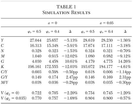
Some back-of-the-envelope calculations can help to interpret the quantitative nature of the paper’s policy experiment. Judson (2012: 25–26) estimates that, as of 2011, $340 billion in $100 and $50 bills were held domestically in the United States, or 40 percent of the $780 billion total in circulation. If large bills have a velocity for unreported cash transactions of 3, and the average (marginal) tax rate is 25 percent, then completely eliminating large notes would add $255.5 billion to U.S. tax coffers, or roughly 1.4 percent of GDP. In my model, reducing φ_τ from 0.5 to 0.4 increases households’ effective tax rate from around 14.5 percent to 16 percent (evaluated at the initial steady-state value of m), a 1.5 percentage point increase. Thus, reducing the semielasticity of money by the amount in this experiment is similar in magnitude to eliminating large bills in the United States.⁹

Consider first the baseline model of panel 1, in which a = 0. Eliminating large-denomination notes (according to the model’s analog) causes households’ effective tax rate to rise from 14.9 percent to 17.3 percent (which is essentially the government’s share of output) and output to decline by over 5 percent. This decline comes about because employment falls by 1.5 percent and capital falls by over 12 percent, owing to the lower incentives to supply inputs in the face of higher marginal tax rates. Not surprisingly, the demand for real money declines, in this case by 12 percent, since cash has less value on the margin after the elimination of large notes. Tax revenues rise, leading to a reallocation of output from the household to the government sector—consumption falls by almost 6 percent and government spending rises by almost 11 percent, with the output share of the former falling slightly.

Given these equilibrium adjustments in response to the policy change, the overall effect on household welfare is negative. As shown by the last rows of the table, steady-state utility falls by 2.2 percent because of the large decline in consumption, while the implied increase in leisure, as labor supply falls, does not offset the consumption effect. If we allow government spending on public goods to directly affect utility with weight of φ_g = 0.035 (10 percent of the weight given to private consumption), the general equilibrium costs of the policy still outweigh the benefits, with welfare declining by 1.7 percent.

Does infrastructure spending by the government improve the case for large-note elimination in the model? The second panel simulates the steady state assuming the parameter a is 5 percent, instead of 0. As might be expected, equilibrium output is higher than the baseline case regardless of the tax evasion parameter, and its decline is also dampened with the policy move, falling by only 1.4 percent. Yet, while the decline in consumption is also weaker than the baseline case, so is the fall in labor supply and the net effect on household welfare remains negative. Even when government spending directly adds to utility, welfare falls with the note-elimination policy by 0.6 percent, noticeably smaller but welfare-reducing nonetheless. The threshold for φ_g in the second parameterization that just makes households indifferent to the policy is a value of 0.2.

Conclusion

This article takes a first step to providing quantitative estimates of the welfare effects of proposals to eliminate currency or large-denomination currency notes in the United States. Importantly, the model is one of general equilibrium, so costs and benefits are clearly specified, coherent, and complete (within the context of the model). My findings indicate that a currency ban might negatively affect overall welfare, which is consistent with the conjectured cautions of Camera (2001: 405).

I have been upfront regarding the many limitations of this study. Models that more precisely distinguish among currencies of different denominations, that incorporate other illicit uses of cash besides tax evasion and allow for alternative transactions media like bitcoin, that more carefully calibrate the model to developed and developing countries, and that pay attention to short-run transitional dynamics are needed before sensible assessments of policy proposals can be made. I leave these important extensions to future work.

Appendix

The complete model, including the household problem and the government budget constraint, and where all functional forms are specified, is given by

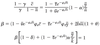
where all variables are as defined in the text. Note that the competitive market model is written in terms of a fictitious central planner where prices are implicit. The functional forms are common. Using standard techniques for optimization yields the following dynamic equilibrium conditions:

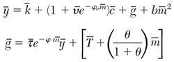
Together with the production function, these equations determine optimal paths for c, n, m, k′, g and y, taking initial values for k and m as given and lump sum taxes, T as exogenous. The model admits a steady state in which the endogenous variables are constant and the rate of inflation π_t = θ. Because T is exogenous, changes in income taxes and seigniorage, which are endogenous, necessarily determine government spending. The model’s steady state is:

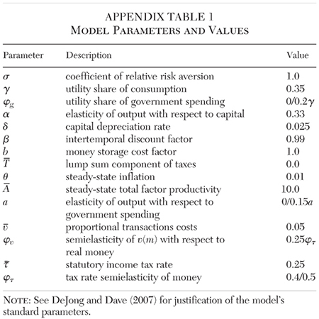
Appendix Table 1 lists the parameters, their description, and the values used in the calibration. As is typical, I assume time is measured quarterly.

References

Alm, J. (2012) “Measuring, Explaining, and Controlling Tax Evasion: Lessons from Theory, Experiments, and Field Studies.” International Tax and Public Finance 19 (1): 54–77.

Balafoutas, L.; Beck, A.; Kerschbamer, R.; and Sutter, M. (2015) “The Hidden Costs of Tax Evasion.” Journal of Public Economics 129: 14–25.

Camera, G. ( 2001) “Dirty Money.” Journal of Monetary Economics 47 (2): 377–415.

Cebula, R. J., and Feige, E. L. (2012) “America’s Underground Economy: Measuring the Size, Growth and Determinants of Income Tax Evasion in the U.S.” Crime, Law and Social Change 57 (3): 265–85.

DeJong, D. N., and Dave, C. (2007). Structural Macroeconometrics. Princeton, N.J.: Princeton University Press.

Gordon, J. P. F. (1990) “Evading Taxes by Selling for Cash.” Oxford Economic Papers 42 (1): 244–55.

Judson, R. (2012) “Crisis and Calm: Demand for U.S. Currency at Home and Abroad from the Fall of the Berlin Wall to 2011.” IFDP Working Paper No. 1058 (November).

Kimball, M. (2017) “Next Generation Monetary Policy.” Journal of Macroeconomics 54: 100–09.

Mazhar, U., and Mon, P. G. (2017) “Taxing the Unobservable: The Impact of the Shadow Economy on Inflation and Taxation.” World Development 90: 89–103.

Rogoff, K. S. (1998) “Blessing or Curse? Foreign and Underground Demand for Euro Notes.” Economic Policy 13 (26): 261–303.

__________ (2016) The Curse of Cash. Princeton, N.J.: Princeton University Press.

Sands, P. (2016) “Making It Harder for the Bad Guys: The Case for Eliminating High Denomination Notes.” M-RCBG Associate Working Paper Series No. 52. Available at https://www.hks.harvard.edu/centers/mrcbg/publications/awp/awp52.

Slemrod, J. (2007) “Cheating Ourselves: The Economics of Tax Evasion.” Journal of Economic Perspectives 21 (1): 25–48.

White, L. H. (2017) “India’s Failed Demonetization Program and Its Retreating Economic Defenders.” Alt-M blog (September 28).

¹Current proposals have been around for a while: Recommendation 24 of the Financial Action Task Force on Money Laundering of the OECD (1998) moves to combat money laundering by “encourag[ing] the replacement of cash transfers” through better money management. More recently, India has demonetized (i.e., removed legal tender status of ) its 500 and 1,000 denomination rupee notes, ostensibly to curb corruption, to mixed reviews (White 2017).

²My model extends the work of Rogoff (1998: Appendix A) to a general equilibrium setting. Rogoff (1998: Appendix B) develops a more realistic model with two currency denominations, but I have used the simpler model here.

³One more reason for my limited focus on tax evasion is that Rogoff (1998: 2) claims that “the effect of curtailing paper currency on tax evasion alone would likely cover the lost profits from printing paper currency, even if tax evasion fell by 10–15 percent.” My approach is one way to directly assess claims like this.

⁴Since my analysis focuses on the economy’s “steady state,” which rules out, by assumption, the possibility of unpredictable shocks, perfect foresight is an innocuous assumption here.

⁵Debt and lump sum taxes are equivalent by the assumptions of Ricardian Equivalence; therefore, I do not model nonmonetary debt explicitly

⁶The economy’s price level will adjust to ensure that real money supply equals real money demand, even if the nominal money stock is exogenously determined by a central bank. Rogoff (1998: 298–99) provides weak conditions for price level determinancy in this model.

⁷The central planner in this model is only an expositional device that has no policy implications. Under the conditions of the model the fictitious planner’s allocation will precisely mimic that of a multiagent, competitive market economy in which prices coordinate choice.

⁸Note the public good nature of government spending—the same quantity can directly add to household utility and improve input productivity.

⁹Rogoff (1998: 60), citing work by Slemrod (2007), notes that the “net tax gap” of uncollected taxes relative to expected taxes was 2.7 percent of U.S. GDP in 2006. The experiment considered here reduces this gap by more than half, which is feasible and plausible. The tax gap estimates in Cebula and Feige (2012) for 2009 in the United States are a bit larger than Slemrod’s.