It is necessary to be clear about what is meant by a state’s preference. The concept explored here is sometimes referred to as a state’s a priori preference. A state prefers a priori the system that results in the greater potential influence of its voters, as represented by the state’s popular-vote majority, on the outcome of an election. In this context the term “a priori” means in consideration of only the system itself, without (a posteriori) considerations of actual or likely outcomes in particular elections (see Felsenthal and Machover 2004.) In addition, as discussed below, a state can be said to prefer an institution only in consideration of and relative to a specific alternative institution.

The analysis here demonstrates (contrary to the existing academic literature) that well over half of the states — in particular the smaller population states — prefer the electoral college.¹ The relationship between state population and electoral college preference derives from the fundamental methods — some described in the Constitution, others in century-old laws — for determining the number of congressional representatives (and consequently the number of electoral votes) assigned to each state. In addition, the inverse relationship between state size and electoral college preference, as well as the majority-of-states preference for the system, have existed throughout the entire history of U.S. presidential elections. Those characteristics are certain to persist for the foreseeable future.

An Overview

The election of the U.S. president is determined by a simple majority vote of the electoral college, the members of which are appointed by the states.² The Constitution directs that the number of electors for each state shall be “equal to the whole Number of Senators and Representatives to which the State may be entitled in the Congress.” The Constitution also directs that the methods for appointing electors and for directing how those electors cast their votes are to be determined by state legislatures.³ At first, electors were selected directly by state legislatures, but the transition to some form of popular vote to decide the assignation of electors proceeded steadily. By 1836 almost all states had changed from state legislature selection of electors to some form of popular vote selection (see Ross 2012: chap. 2; Miller 2012).

The first electoral college, for the election of 1788, consisted of 69 electors across the 10 states that by then had ratified the Constitution. The electoral college increased in size monotonically, in accordance with the increase in the number of senators and representatives, reaching its current size of 538 with the election of 1964. The number of senators has been at 100 since the admission of Hawaii and Alaska to the Union in 1959. The number of representatives has been capped at 435 since the Apportionment Act of 1911.⁴ The District of Columbia has neither senators nor representatives, but was granted three electoral votes in accordance with Amendment XXIII to the Constitution, ratified in 1961. Hence, the current total of 538 electoral votes.

Because every state has two senators and at least one representative, every state has at least three electoral votes. As of 2016 each of the seven smallest states, as well as the District of Columbia, has three electoral votes; the largest state, California, has 55. The median is eight electoral votes. Unless a new state is added or Congress revises the number of representatives (something it has not done in over 100 years), the current total of 538 electoral votes will prevail.

Unanimity versus Maine and Nebraska

Regardless of who was doing the selecting — state legislatures or some subset of the population — electors have been directed, with few exceptions, to cast their state’s electoral votes for president unanimously: winner take all. From 1788 through 2016, there have been 58 presidential elections and 2,238 state electoral vote tabulations for the office of president of the United States; 2,186 of the 2,238 tabulations, 97.7 percent, have been unanimous. The lack of unanimity in the 2.3 percent of vote tabulations could have resulted from an explicit nonunanimous allocation method chosen by a state, or from a so-called faithless elector: one who casts a vote in violation of a state’s voting rules.⁵

In any case, the dominance of a winner-take-all allocation should not be surprising. Once the majority’s preference is determined, that majority would presumably want to maximize the state’s influence on the final outcome, which is accomplished with the winner-take-all allocation of electoral votes.

Nonetheless, Maine (four electoral votes) and Nebraska (five electoral votes) have opted out of winner take all, in favor of the “congressional district” method. Under that method the popular vote winner in each congressional district receives that district’s electoral vote; the popular vote winner in the state receives the two “senatorial” electoral votes. Maine adopted the congressional district method in advance of the 1972 election and Nebraska in advance of the 1992 election.⁶

When a state splits its electoral votes (as both Maine and Nebraska have done), the influence of the state’s majority on the outcome of the election is diminished. Thus, whatever the reasons for those two states to have adopted the congressional district method, it is not likely that their example will be followed by any significant number of other states. In sum, the obvious benefit of unanimity explains why so few states have ever chosen the congressional district or any other nonunanimous method for the allocation of their electoral votes.

Electoral College Influence and Popular Vote Influence

Let e_i represent the electoral votes in state i, which are all allocated to the winner of the popular vote in the state (with few exceptions, as noted). Thus, each state’s proportional contribution to the electoral vote is:

(1)

conditional only on the winner of the popular vote in the state. I will use E_i as the measure of a state’s electoral vote influence. (Other measures of influence are considered below, but as a starting point I focus on shares.)

Now consider the distribution of popular vote influence across the states. At first, a state’s popular vote influence might seem to be an artificial construct. Each vote counts the same toward the national popular vote regardless of the voter’s place of residence. Nonetheless, the state remains the relevant locus because whether a state prefers the electoral college can only be determined by the state and in consideration of an alternative. In particular, I analyze the most commonly suggested and plausible alternative — namely, whether a state would prefer to have the election determined by the electoral college or by the national popular vote. To answer that question it is assumed that a state will prefer the system that maximizes the potential influence of its voters, as represented by the state’s popular vote majority, on the outcome of an election.

With regard to a state’s popular vote influence, it will help to define some basic measures. Start with two political parties, designated as the D party and the R party.

(2)	: votes for the D party in state i

(3)	: votes for the R party in state i

(4)	: the positive vote difference (the margin) between the parties in state i, which is accorded to the winning party

(5)	: the vote total in state i

For each state the popular vote margin in percentage terms is the difference in the vote between the two parties, relative to the total votes cast:

(6)	: state i’s percentage popular vote margin.

With

(7)	: state i’s share of the national vote,

it follows that the difference in the total vote within a state relative to the total vote in the country is given by

(8)

Thus, every state’s contribution to the national popular vote margin is the popular vote margin in the state multiplied by the relative size of the state. In terms of the popular vote, the state margin and state size are multiplicative. And not surprisingly, abstracting from the margin (an a posteriori concept), each state’s share of the national population (β_i) is a direct measure of its potential (a priori) influence on the election under a national popular vote.

State Preferences: 2016

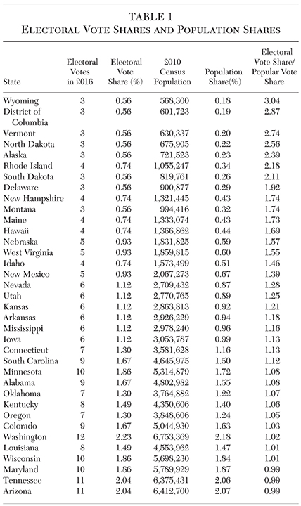
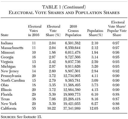
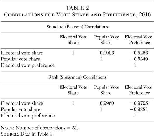
The electoral vote shares and the population shares for each state are shown in Table 1.⁷ The correlations for the various metrics are shown in Table 2.⁸ Population shares and electoral shares are almost perfectly correlated. The more interesting value, however, is the ratio of the two shares. That ratio, with the electoral vote share as the numerator, can be described as the electoral college preference or simply the “electoral preference”:

(9)

(10)

An electoral preference greater than one means that the state’s electoral vote share is greater than its popular vote share, and vice versa. This ratio offers a simple and direct indicator of a state’s a priori preference for the electoral college. In 2016, 32 states and the District of Columbia had an electoral preference greater than one. The median electoral preference was 1.08. The distribution of electoral preferences across states is shown in Table 1 and Figure 1.

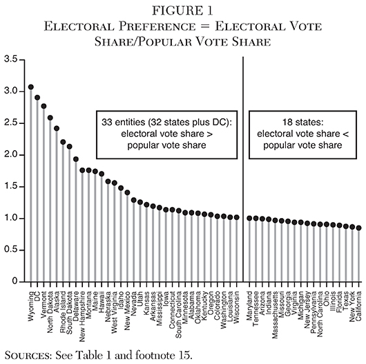
The states with an electoral preference greater than one are overwhelmingly the smaller states. Indeed, electoral preference is largely a function of state population. The rank correlation between population shares and electoral preference is 20.988; the two measures produce almost identical (inverse) rankings. That relationship between electoral preference and population share, shown in Figure 2, results in the characteristic hyperbolic form.

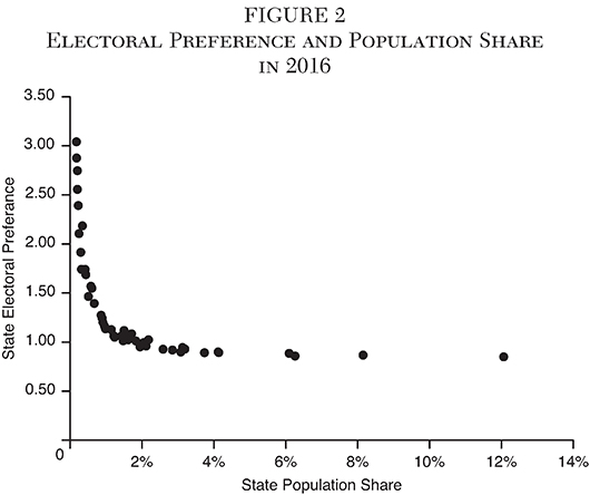
The inverse relationship between population and electoral preference derives from the method used to determine the number of congressional representatives per state, which determines the number of electors per state. As already described, each state has two senators and at least one representative, so each state has at least three electoral votes. The remaining 385 representatives — and their electoral votes — are allocated among the remaining states based on population, as described in the next section.

Apportioning the House of Representatives

In accordance with the Constitution, the House of Representatives is reapportioned every 10 years (see U.S. Constitution, Article I, Sections 2 and 3). The reapportionment occurs with the second full congressional term following the publication of the decennial census. For example, the composition of the 112th Congress (2011–12 term) was the last apportioned according to the 2000 census. The 113th Congress (2013–14 term) was the first apportioned according to the 2010 census. As noticed earlier, the total number of representatives has been capped at 435 since 1911. The 385 additional representatives (beyond the minimum of one per state) are apportioned by state population, according to the schedule just described.

Several different apportioning methods have been used since the first census in 1790. The current method has been in place since 1941 and is known as the “equal proportions method.” The method appears to have been suggested by the mathematician Edward Huntington and by Joseph Hill, Chief Statistician of the Bureau of Census. Sometimes referred to as the Huntington-Hill method, it is applied as follows.⁹

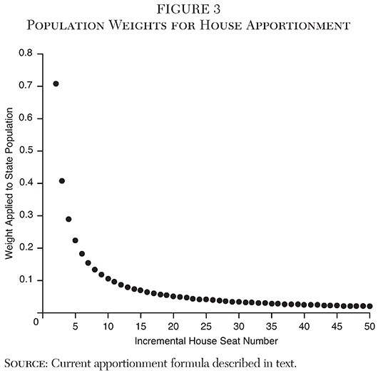
Each additional representative (house seat) is given a weight:

(11)

Where n represents the number of seats a state would have if it gained a seat. Because all states automatically receive one seat, the first seat gained is seat two. The weight for seat two is

(12)

the weight for seat three is

(13)

and so on. The weights are shown in Figure 3. The weighting formula reflects, indeed it can be said to generate, the relationship between electoral preference and population shown in Figure 2.

The weights are multiplied by the state populations (P_i) to create a series of values (H_n,i) for seat n, for each state i:

(14)

A sufficient number of the H_n,i values, say 99, are calculated for each state: Alabama H(2) through Alabama H(100); Alaska H(2) through Alaska H(100); and so on. (The number of values created for each state needs only to exceed by one the number of seats eventually granted to the largest state.) The resulting values are then sorted from highest to lowest. The first 385 values of that sorted sequence determine the additional seats received by each state.

The above formula for allocating those 385 additional representatives, along with the three-vote minimum for each state, generates the result described here: small states will have high electoral shares relative to their population shares, while the inverse holds for large states.

The Conventional View

While the issue is not always clearly presented, the general consensus in the academic literature appears to be that the electoral college system reflects and maintains the inherent advantage of large states.¹⁰ That analysis begins with the insightful distinction between voting share and voting power in systems with unequal voting shares, such as the electoral college.¹¹

Voting power derives from the likelihood that a voter will be influential, in the sense that changing just that one vote would change the outcome of the election. That likelihood is determined not just by a voter’s share, but by the distribution of all voting shares. While voting power will generally be highly correlated with voting share, the two concepts are not necessarily equal and can, under certain circumstances, be quite different. As a simple example, if a single entity controls more than half of the voting shares in a simple majority election, then only that entity’s vote matters. Its voting power is measured as one, and any other entity’s voting power is measured as zero, regardless of the specific shares.

Two commonly used measures of voting power are the Banzhaf index (sometimes referred to as the Penrose-Banzhaf index) and the Shapley-Shubik index. The Banzhaf index for a voter is calculated by creating all possible winning coalitions, of any size, and then calculating the percentage of those winning coalitions in which the voter at issue casts an influential vote — a vote that if changed would change the outcome of the election. Because any particular coalition can have multiple influential voters, the Banzhaf index must be normalized to sum to one.

The Shapley-Shubik index for a voter is calculated by creating all possible sequences of all of the voters and then calculating the percentage of those sequences in which the voter at issue casts the deciding vote, assuming that all prior voters in the sequence voted in the same way (that is, as a coalition). Every sequence will have only one deciding voter, the one who “tips the scales” when the votes are tabulated sequentially.¹²

We now compare these two indices with the population share calculations from Table 1. Table 3 displays the correlations among (1) the electoral vote shares and the two electoral vote power indices, (2) the population shares and the two population power indices, and (3) the electoral preference ratios derived from the shares and the two power indices.¹³

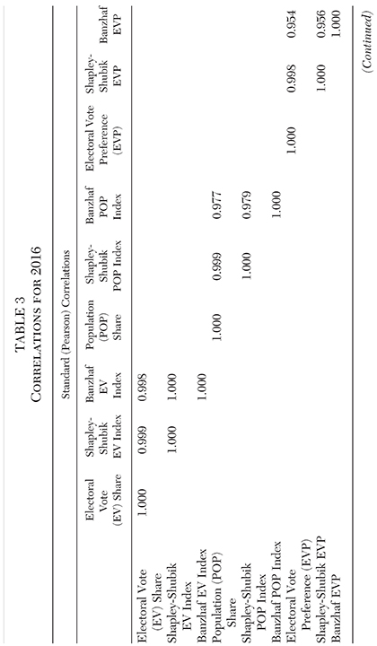
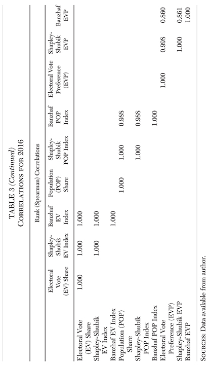
When it comes to the electoral college and state populations, shares and power indices are highly correlated (the lowest standard correlation is 0.977) and tend to produce similar rankings (the lowest rank correlation is 0.988). Although some mid-size states switch their electoral preference from one side of 1.0 to the other, based on share versus power index, the electoral preference values are also highly correlated. The lowest standard correlation is 0.954; the lowest rank correlation is 0.860.

In addition, the median electoral preference is 1.08 based on shares, 1.17 based on the Banzhaf index, and 1.09 based on the Shapley-Shubik index. The number of states (and the District of Columbia) with an electoral vote preference greater than 1.0 is 33 based on shares, 36 based on the Banzhaf index, and 34 based on the Shapley-Shubik index. When it comes to measuring electoral college influence, popular vote influence, or the electoral preference of the states, it makes no substantive difference whether we use shares or one of the power indices.

In any case, because electoral voting shares and electoral voting power both favor the larger states, the existing literature generally sees the electoral college as reflecting and maintaining the inherent large-state advantage that size confers.¹⁴ That straightforward observation about the advantage of size is, however, uninformative about a state’s preference for one system over the other.

Recall the question that we are attempting to answer: Assuming that a state wants to maximize the a priori influence of its voters, as represented by the popular vote majority, would that state prefer to have the election determined by the electoral college or by the national popular vote? The existing literature gets the answer wrong because it takes the greater influence of large states — inherent in both the electoral college and the national popular vote — as dispositive, without making the appropriate comparison between the two systems. That is, the existing literature fails to compare the state’s electoral college influence relative to the influence the state would have in a national popular vote. The analysis here measures that relative influence and thereby identifies which system would be preferred a priori by the voters in any given state.

State Preferences: 1788–2012

The current distribution of populations and electoral votes implies that the majority of states — in particular, the smaller ones — prefers the electoral college system. Has that pattern always prevailed? Computing the same values (as shown in Table 1 for the 2016 election) over all of the presidential elections is straightforward. To arrive at populations for an election year, I interpolate between decennial census figures. The 1790 census is used to measure population shares for 1788. The 2010 census is used to measure population shares for 2012.¹⁵

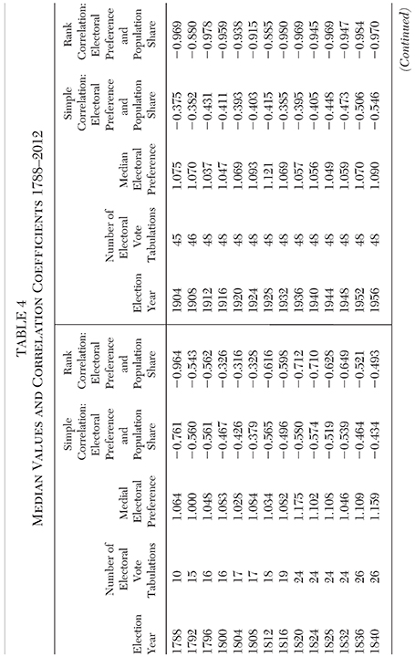
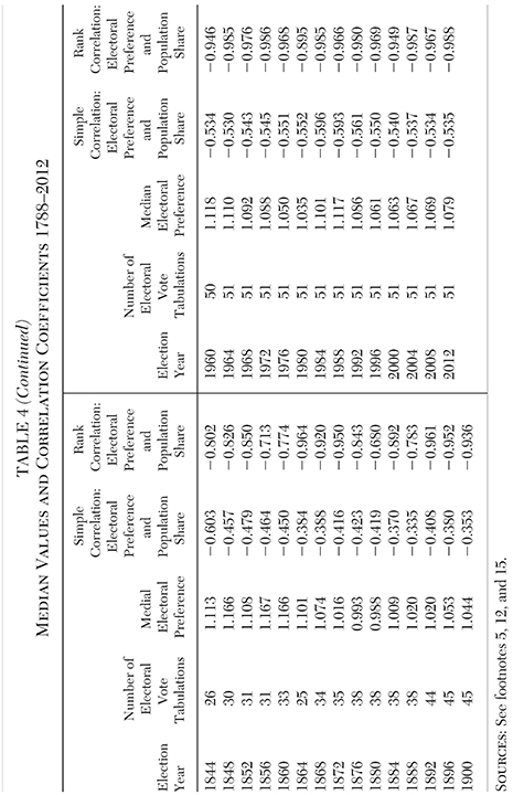
Measuring the electoral college shares from reported tabulations and the population shares from the census figures generates the results shown in Table 4. In only two of the 58 presidential elections (1876 and 1880) has the median electoral preference been lower than one. In all of the other elections the majority of the states have, by this measure, preferred the electoral college system. In addition, the strong negative relationship between electoral preference and population has always prevailed; both the simple and the rank correlations between electoral preference and population have always been significantly negative. The empirical results indicate that the current method of apportionment (in effect since 1941) did not fundamentally alter the relationship between state population and electoral preference; that relationship has always existed.

It should also be noted that there is nothing inevitable about the majority of states preferring the electoral college. It is possible to describe a distribution of populations such that the majority of states would prefer a popular vote. Such an outcome would occur, for example, if the distribution of state populations were bimodal, with a group of similar small population states and a group of similar large population states, with the number of small states less than the number of large states. For example, consider if there were 20 states with small populations (20 states like, say, Wyoming) such that each was accorded the minimum number of electors, with the remaining population and electors divided among the 30 other states (30 states like, say, Florida). That distribution of populations and the implied distribution of electoral votes could generate a majority of states in favor of a popular vote system.

Conclusion

There is a powerful reason for the persistence of the electoral college: a majority of states — overwhelmingly the smaller ones — prefer it, which has been the case throughout U.S. history. Furthermore, abandoning the electoral college can only happen through constitutional amendment, which requires the assent of not just a majority but three-fourths of the states (see U.S. Constitution, Article V). Given the structure of the electoral college and the distribution of state populations, such an outcome is implausible in the foreseeable future.

The distribution of congressional representatives (and consequently of electors) was not happenstance, but rather the result of a purposeful compromise among the states, in consideration of the wide variation in state populations. The Constitution embodies several such accommodations, so as to prevent a small number of large states from dominating political outcomes. As one of those accommodations, the electoral college is likely to remain durable.

References

Abbott, D. W., and Levine, J. P. (1991) Wrong Winner: The Coming Debacle in the Electoral College. Westport, Conn.: Praeger.

Banzhaf, J. F. (1965) “Weighted Voting Doesn’t Work.” Rutgers Law Review 19: 317–43.

— — — — — (1968) “One Man, 3.312 Votes: A Mathematical Analysis of the Electoral College.” Villanova Law Review 13: 304–32.

Bhattacharyya, G. K., and Johnson, R. A. (1977) Statistical Concepts and Methods. New York: Wiley.

Boylan, T. S. (2008) “A Constitutional Defense of the Electoral College and the Election of the American President.” The Open Political Science Journal 1: 50–58.

Farrand, M., ed. (1937) The Records of the Federal Convention of 1787. New Haven, Conn.: Yale University Press.

Felsenthal, D. S., and Machover, M. (2004) “A Priori Voting Power: What Is It All About?” Political Studies Review 2: 1–23.

— — — — — , eds. (2012) Electoral Systems: Paradoxes, Assumptions, and Procedures. New York: Springer.

Gelman, A.; Katz, J. N.; and Bafumi, J. (2004) “Standard Voting Power Indices Do Not Work: An Empirical Analysis.” British Journal of Political Science 34: 657–74.

Gelman, A.; Katz, J. N.; and Tuerlinckx, F. (2002) “The Mathematics and Statistics of Voting Power.” Statistical Science 17: 420–35.

Gelman, A.; Silver, N.; and Edlin, A. (2012) “What Is the Probability Your Vote Will Make a Difference?” Economic Inquiry 50: 321–26.

Gibson, C., and Jung, K. (2002) “Historical Census Statistics on Population Totals by Race, 1790 to 1990, and by Hispanic Origin, 1790 to 1990, for the United States, Regions, Divisions, and States.” Washington: U.S. Census Bureau.

Gregg, G. L., ed. (2001) Securing Democracy: Why We Have an Electoral College. Wilmington, Del.: ISI Books.

Hamilton, A.; Madison, J.; and Jay, J. ([1788] 1961) The Federalist Papers. New York: New American Library.

Huntington, E. V. (1921) “The Mathematical Theory of the Apportionment of Representatives.” Proceedings of the National Academy of Sciences 7: 123–27.

— — — — — (1928) “The Apportionment of Representatives in Congress.” Transactions of the American Mathematical Society 30: 85–110.

Katz, J. N.; Gelman, A.; and King, G. (2004) “Empirically Evaluating the Electoral College.” In A. N. Crigler et al. (eds.) Rethinking the Vote: The Politics and Prospects of American Election Reform. Oxford: Oxford University Press.

Kimberling, W. C. (1992) “The Electoral College.” Federal Election Commission.

Kuroda, T. (1994) The Origins of the Twelfth Amendment: The Electoral College in the Early Republic, 1787–1804. Westport, Conn.: Greenwood Press.

Leech, D. (2002a) “An Empirical Comparison of the Performance of Classical Power Indices.” Political Studies 50: 1–22.

— — — — — (2002b) “Computation of Power Indices.” University of Warwick, Economic Research Paper No. 644.

Longley, L. D., and Peirce, N. R. (1996) The Electoral College Primer. New Haven, Conn: Yale University Press.

Madison, J. ([1840] 1987) Notes of Debates in the Federal Convention of 1787. New York: Norton.

Mann, I., and Shapley, L. S. (1964) “The A Priori Voting Strength of the Electoral College.” In M. Shubik (ed.) Game Theory and Related Approaches to Social Behavior. Hoboken: N. J.: Wiley.

Margolis, H. (1983) “The Banzhaf Fallacy.” American Journal of Political Science 27: 321–26.

Miller, N. R. (2009) “A Priori Voting Power and the U.S. Electoral College.” Homo Oeconomicus 26: 341–80.

— — — — — (2012) “Why the Electoral College Is Good for Political Science (and Public Choice).” Public Choice 150: 1–25.

Penrose, L. S. (1946) “The Elementary Statistics of Majority Voting.” Journal of the Royal Statistical Society 109: 53–57.

Rabinowitz, G., and MacDonald, S. E. (1986) “The Power of the States in U.S. Presidential Elections.” American Political Science Review 80: 65–87.

Ross, T. (2012) Enlighted Democracy: The Case for the Electoral College. 2nd edition. Clinton, Mass.: Colonial Press.

Saari, D. G. (1978) “Apportionment Methods and the House of Representatives.” American Mathematical Monthly 85: 792–802.

Shapley, L. S., and Shubik, M. (1954) “A Method for Evaluating the Distribution of Power in a Committee System.” American Political Science Review 48: 787–92.

Strömberg, D. (2008) “How the Electoral College Influences Campaigns and Policy: The Probability of Being Florida.” American Economic Review 98: 769–807.

¹ The general consensus in the academic literature appears to be that the electoral college system reflects and maintains the greater influence of large states. For example, see Banzhaf (1965, 1968), Rabinowitz and MacDonald (1986), Strömberg (2008), and Miller (2009, 2012).

² Comprehensive and relatively recent (since 1990) treatments of the history, purpose, and effects of the electoral college are found in books by Abbot and Levine (1991), Kuroda (1994), Longley and Peirce (1996), Gregg (2001), and Ross (2012). Helpful overviews and bibliographies can also be found in articles by Kimberling (1992), Boylan (2008), Strömberg (2008), and Miller (2012). The original texts and documents are The Constitution of the United States of America as Amended (Article II, Amendment XII, and Amendment XXIII), The Federalist Papers (39 and 68), The Records of the Federal Convention of 1787, and James Madison’s Notes of Debates in the Federal Convention of 1787.

³ Article II, Section 1 of the Constitution states in part: “Each State shall appoint, in such a Manner as the Legislature thereof may direct, a Number of Electors, equal to the whole Number of Senators and Representatives to which the State may be entitled in the Congress.” Two amendments to the Constitution relate to the electoral college. Amendment XII (ratified in 1804) clarifies several aspects of the electoral college system (in particular requiring each electoral vote to indicate choices for both a president and a vice president, as well as clarifying the method of selecting a president in the event that no candidate obtains a majority of the electoral votes). Amendment XXIII (ratified in 1961) assigns three electoral votes to the District of Columbia.

⁴ The 435 maximum was further codified by the Permanent Apportionment Act of 1929. (With the admission of Alaska and Hawaii to the Union the number of representatives increased temporarily to 437, until the subsequent reapportionment.) Each state has at least one representative and the remaining 385 (5 435–50) are apportioned among the states as a function of their populations. State populations are determined by the decennial census, as prescribed in the Constitution: see Article I, Section 2. Reapportionment of the House also occurs every 10 years, as prescribed in the Constitution: see Article I, Section 3.

⁵ Of course, states with nonunanimous rules can also generate unanimous outcomes. Seldom have states adopted such rules, however, as discussed below. The National Archives and Records Administration reports the electoral college tabulations for every presidential election. The tabulations can be found at www.archives.gov/federal-register/electoral-college/votes.

⁶ I have seen conflicting accounts of whether any other states have ever adopted nonunanimous elector allocation methods, but if so those methods were subsequently rescinded.

⁷ In order to have a consistent population measure across all elections, the decennial census data are used to measure population shares. State population shares are, of course, only approximations for the shares of eligible voters, but the correlation should be very high.

⁸ The correlation tables show both standard (Pearson) correlations and rank (Spearman) correlations. Standard and rank correlations are calculated with analogous formulae, except that rank correlations are derived after replacing the values of the variable pairs by their rank order, 1 through n, from highest to lowest (see Bhattacharyya and Johnson 1977: chaps. 12 and 15).

⁹ See Huntington (1921, 1928) and Saari (1978). Helpful discussions can also be found at: www.census.gov/history/www/reference/apportionment/methods_of_apportionment.html; www.census.gov/population/apportionment/about/computing.html; and www.history.house.gov/home.

¹⁰ See the articles cited in footnote 1. As shown here, the small state advantage in the electoral college derives from the relationship between popular vote shares and electoral vote shares. While that relationship is sometimes described in the literature, its relevance is overlooked. Strömberg (2008) and Gelman, Silver, and Edlin (2012) might be considered exceptions, but their conclusions derive from a posteriori analysis of particular elections. I have been unable to identify any academic research that defines and quantifies the state-by-state preference for the electoral college and the resulting small state advantage, as I do here. The literature on this subject is vast, however, so that contention may be incorrect.

¹¹ Regarding such systems, scholars long ago began to distinguish between voter share and voter power. The seminal articles are Penrose (1946), Shapley and Shubik (1954), Mann and Shapley (1964), and Banzhaf (1965, 1968). For helpful surveys, see Leech (2002a, 2002b), Felsenthal and Machover (2004, 2012), and Strömberg (2008).

¹² An accessible discussion of the two indices is found at www.math.colostate.edu/~spriggs/m130/power2.pdf. The indices herein are calculated using computational methods provided by the University of Warwick at http://homepages.warwick.ac.uk/~ecaae/index.html.

¹³ The data underlying the correlations are available from the author.

¹⁴ The existing literature adds a second step to the analysis such that the electoral power index is adjusted by a corresponding voter power index. That is, the likelihood that an individual voter in a given state will cast an influential vote (the likelihood that the popular vote is tied) is factored into the analysis. The probability of a tie vote, however trivial, is inversely related to population — smaller in larger states and vice versa. The result is that the substantial advantage for large states inherent in the electoral college is reduced to some extent, but not enough to overcome that advantage. Miller (2012) summarizes that analysis:

An individual’s voting power is the probability that his vote is decisive within the state times the probability that his state’s bloc of electoral votes is decisive in the Electoral College. . . . This effect, first noted with explicit reference to the Electoral College by Banzhaf (1968) . . . and it implies that voters in the most favored state (California) have almost three and half times the voting power as voters in the least favored state (Montana, the largest with only one House seat).

Criticism of this two-stage analysis can be found in Margolis (1983), Gelman et al. (2002, 2004, 2012), and Katz, Gelman, and King (2004). The two-stage analysis is not relevant here (or at all, some might argue) because our interest is in the preference of the state as represented by the majority of the voters in the state.

¹⁵ The decennial census data can be found at: www.census.gov/population/www/censusdata/pop1790-1990.html; www.census.gov/population/www/cen2000/maps/respop.html; and www.census.gov/population/apportionment/data/2010_apportionment_results.html. For 1790 through 1860, the population figures reflect the decennial census “free” population as calculated by Gibson and Jung (2002). In any given election year, a state’s population is used (to calculate total population and state shares) only if there is an electoral vote tabulation for that state in the National Archives and Records Administration database.